Links
AI / Agents
Developers
Community
Contributing guide
Full license Apache-2.0
Meta
Requires: Python >=3.12
Provides-Extra: dataframes, optax, blackjax, dev, docs, cuda, all, all_cuda
Package Info
NumPyro Forecast



Bayesian time series forecasting with plain NumPyro models. numpyro_forecast is a functional, JAX-native port of the ideas in Pyro’s pyro.contrib.forecast: you write the generative model as a NumPyro function (covariates, data=None) from a few building blocks, and the package handles the train/forecast split, prediction, backtesting and scoring. Inference is whatever NumPyro (SVI, MCMC) or BlackJAX you write, and the same code runs on CPU or GPU with one numpyro.set_platform call.
📖 Documentation: https://juanitorduz.github.io/numpyro_forecast/
📚 Examples: many worked notebooks, from univariate and hierarchical forecasting to intermittent demand, state space models and VAR: https://juanitorduz.github.io/numpyro_forecast/docs/examples/
Arrays follow Pyro’s layout: time at axis -2, the observation dimension at -1, batch dimensions to the left. Univariate, multivariate and hierarchical models all fit that layout. It is not an AutoML library: there is no model zoo, you define the model and the package gives you a clean path from model to forecasts and scores.
Related project: PyMC-Forecast carries the same ideas over to PyMC with a class-based API. Pick it when your models live in PyMC.
Installation
Requires Python >= 3.12.
uv add numpyro_forecast
# or, with pip:
pip install numpyro_forecast
Optional extras:
dataframes: pandas and polars, so results_to_dataframe can flatten backtest results.optax: optax optimizers for SVI, wrapped withnumpyro.optim.optax_to_numpyro.blackjax: the BlackJAX kernels and Pathfinder innumpyro_forecast.contrib.blackjax.cuda: the CUDA jax plugin (Linux only), see Scaling to GPU.- all: the three above plus the
devanddocstooling (all_cudaaddscuda). Thedocsextra also installsdynestyxfor the dynestyx state space model integration example; without it, that one notebook needspip install "dynestyx>=0.5.1".
Quickstart
Define a model, fit it with SVI, and draw probabilistic forecasts:
>>> import jax.numpy as jnp
>>> import numpyro
>>> import numpyro.distributions as dist
>>> from jax import random
>>> from numpyro.infer import SVI, Trace_ELBO
>>> from numpyro.infer.autoguide import AutoNormal
>>> from numpyro.infer.reparam import LocScaleReparam
>>> from numpyro.optim import Adam
>>> from numpyro_forecast import (
...     Horizon, draw_posterior, eval_crps, forecast, innovations, predict
... )
>>> from numpyro_forecast.features import fourier_features
...
>>> def seasonal_model(covariates, data=None):
...     """Local-level random walk + Fourier seasonality, Student-T noise."""
...     h = Horizon.from_data(covariates, data)
...     num_features = covariates.shape[-1]
...     bias = numpyro.sample("bias", dist.Normal(0.0, 10.0))
...     weight = numpyro.sample(
...         "weight", dist.Normal(0.0, 0.1).expand([num_features]).to_event(1)
...     )
...     drift_scale = numpyro.sample("drift_scale", dist.LogNormal(-3.0, 1.0))
...     sigma = numpyro.sample("sigma", dist.LogNormal(-2.0, 1.0))
...     nu = numpyro.sample("nu", dist.Gamma(10.0, 2.0))
...     # In-sample innovations at "drift", the forecast suffix at "drift_future".
...     drift = innovations(h, "drift", dist.Normal(0.0, drift_scale), reparam=LocScaleReparam(0))
...     level = jnp.cumsum(drift, axis=-2)  # random-walk level
...     regression = (weight * covariates).sum(axis=-1, keepdims=True)
...     prediction = level + bias + regression
...     # Registers "obs" over the training window and "forecast" over the horizon.
...     predict(h, dist.StudentT(df=nu, loc=0.0, scale=sigma), prediction)
...
>>> # Synthetic weekly-seasonal series: time at axis -2, one observation dim at -1.
>>> period, t_obs, horizon = 52.0, 156, 26
>>> duration = t_obs + horizon
>>> covariates = fourier_features(duration, period=period, num_terms=3)
>>> t = jnp.arange(duration)[:, None]
>>> truth = jnp.sin(2 * jnp.pi * t / period) + 0.01 * t
>>> data = truth[:t_obs]
>>> key_fit, key_post, key_pred = random.split(random.PRNGKey(0), 3)
>>> guide = AutoNormal(seasonal_model)
>>> svi = SVI(seasonal_model, guide, Adam(step_size=0.01), Trace_ELBO())
>>> svi_result = svi.run(key_fit, 1_500, covariates[:t_obs], data, progress_bar=False)
>>> posterior = draw_posterior(key_post, guide, svi_result.params, num_samples=100)
>>> samples = forecast(key_pred, seasonal_model, posterior, data, covariates)
>>> samples.shape  # (draws, horizon, obs)
(100, 26, 1)
>>> bool(eval_crps(samples, truth[t_obs:]) < 1.0)
True
samples holds the forecast draws over the held-out horizon, shaped (sample, *batch, future, obs): one row per posterior draw, ready for eval_crps and the rest of the evaluation helpers. The horizon is whatever covariates has beyond data.
The examples on this page are executed by the test suite (pytest --doctest-glob=README.md), so they are always current.
Model building blocks
A model is a plain NumPyro function (covariates, data=None) whose first line derives its Horizon from the shapes. The building blocks are ordinary functions that call numpyro.sample and numpyro.deterministic for you against that horizon:
| Building block | What it does |
|---|---|
Horizon.from_data(covariates, data) |
Derives the train/forecast split (t_obs, future, duration) from the shapes |
innovations(h, name, prior) |
Samples iid per-step innovations outside any loop; you build the series from them (a random walk is jnp.cumsum(drift, axis=-2)) |
markov_series(h, name, init_carry, transition) |
Samples one step at a time inside scan, for per-step distributions that depend on the previous state |
ssoe(h, name, y, init_carry, mean, update, noise_dist) |
Single-source-of-error recursion (ARMA, exponential smoothing, Croston, TSB): an iid error plate driving a deterministic filter |
predict(h, obs_dist, prediction) |
Conditions the observation distribution on the training window (obs) and samples the horizon (forecast) |
One model both trains and forecasts. In-sample latents live at <name> and the forecast horizon at a separate <name>_future site that the guide never sees, so AutoNormal never resizes and Predictive draws the suffix from the prior. A vector autoregression is an ssoe recursion with the mean/update pair from numpyro_forecast.var and the Minnesota prior moments from numpyro_forecast.priors; see the VAR example.
Inference
Nothing in the package wraps svi.run or mcmc.run. Fit the model with any of:
- SVI with any NumPyro autoguide (
AutoNormal,AutoMultivariateNormal, …) and any NumPyro or optax optimizer. - MCMC with any kernel: NumPyro’s
NUTS, or the BlackJAX kernels BlackjaxNUTSKernel, BlackjaxMCLMCKernel and BlackjaxCustomKernel fromnumpyro_forecast.contrib.blackjax, plainMCMCKernels you hand toMCMC. - Pathfinder via fit_multipathfinder and multipathfinder_samples, also in
numpyro_forecast.contrib.blackjax.
Every driver (forecast, predict_in_sample, to_datatree, backtest) takes a plain dict of posterior draws, so mcmc.get_samples(), draw_posterior for a variational guide and the Pathfinder samplers are interchangeable. The inference methods comparison fits one model with NUTS, SVI, Pathfinder and MCLMC and scores their forecasts side by side. The quickstart model, fitted with NUTS instead of SVI:
>>> from numpyro.infer import MCMC, NUTS
...
>>> mcmc = MCMC(
...     NUTS(seasonal_model), num_warmup=500, num_samples=500, num_chains=1, progress_bar=False
... )
>>> mcmc.run(key_fit, covariates[:t_obs], data)
>>> samples = forecast(key_pred, seasonal_model, mcmc.get_samples(), data, covariates)
>>> samples.shape
(500, 26, 1)
Time-axis reparameterization
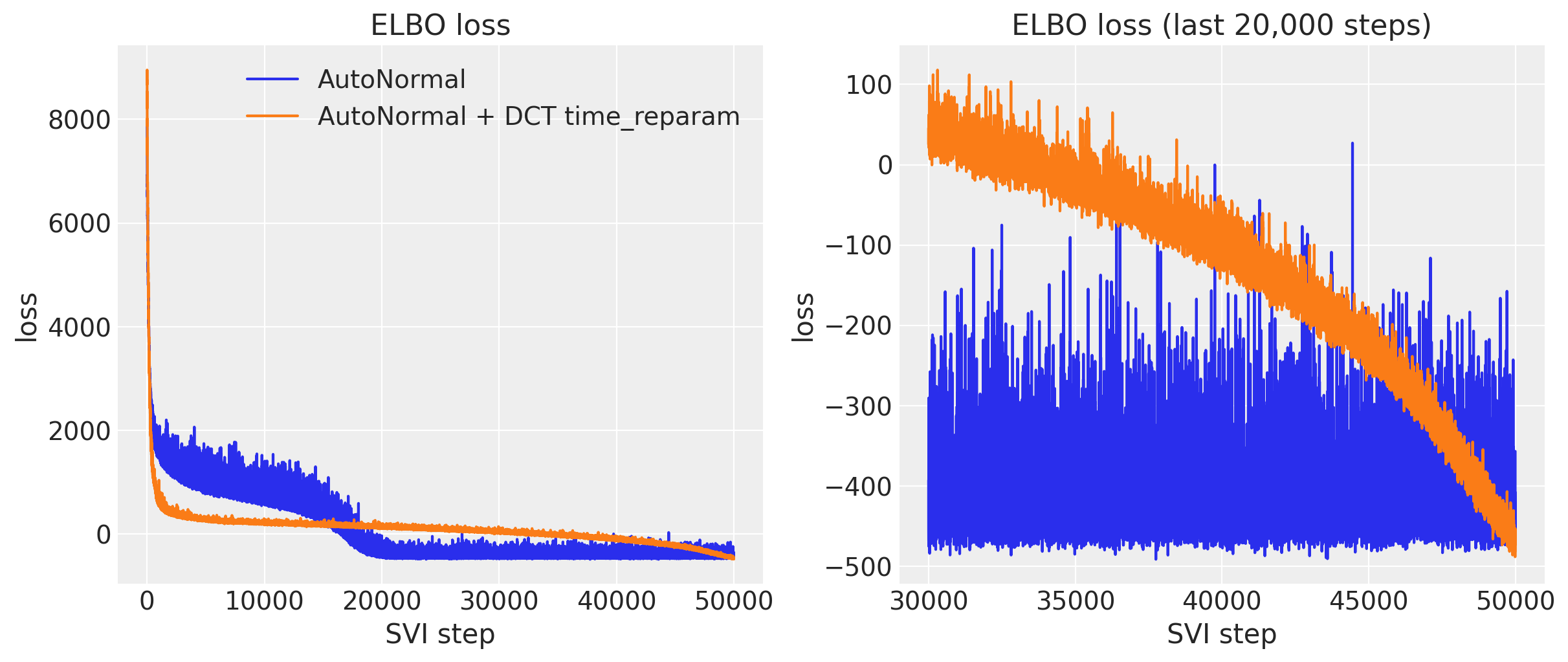
time_reparam(model, "haar" | "dct") is the port of the time_reparam option of Pyro’s Forecaster. It wraps the model with handlers.reparam so every in-sample innovations site is sampled in a Haar wavelet or discrete cosine basis. The rotation has unit Jacobian, so the model and its posterior are unchanged; only the geometry the guide or sampler sees changes, from strongly correlated increments to nearly independent coefficients. Create the wrapped model once and hand that same object to the guide, to SVI or MCMC and to the drivers. On the random-walk level of the univariate example, a mean-field AutoNormal reaches a lower ELBO loss in the DCT coordinates:
Backtesting and evaluation
backtest(rng_key, model_fn, data, covariates, forecast_fn=...) runs the rolling or expanding window loop and scores every window. Fitting and forecasting are closures you write, so backtest does not depend on how a model is fit; backtest_vectorized fits every rolling window in one vmapped SVI run. The metrics are eval_crps, eval_mae, eval_rmse and eval_coverage, plus crps_empirical, eval_pinball, eval_interval_score and make_mase in numpyro_forecast.metrics; evaluate_forecast bundles them. to_datatree exports a posterior with its in-sample predictive, forecasts and observed data as an ArviZ-schema xarray.DataTree for diagnostics and plotting.
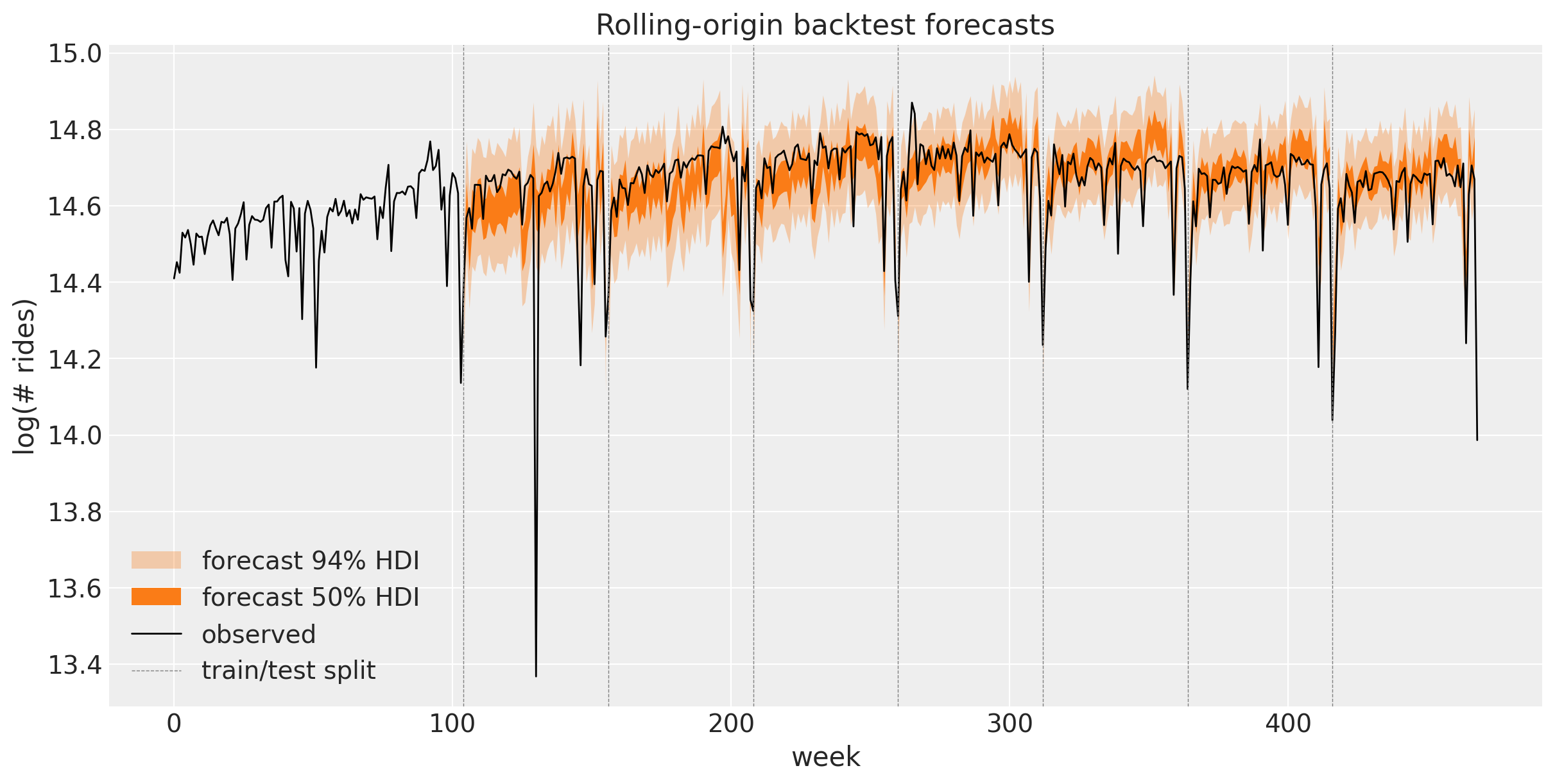
Rolling-origin backtest from the univariate example: every window refits the model and forecasts the next block, shown with its 50\% and 94\% HDI bands.
Scaling to GPU
Everything is plain JAX. Install the cuda extra and select the platform before fitting; the model, the inference code and the drivers do not change:
import numpyro

numpyro.set_platform("cuda")
On an accelerator the posterior draws are usually the largest allocation, so draw_posterior, forecast, predict_in_sample and to_datatree take batch_size to chunk the sample axis and device="host" to move each chunk off the accelerator as it is drawn (to_datatree defaults to "host"; backtest forwards batch_size to your closures). The stockout example fits a 1,000-series retail panel with SVI and a custom optax optimizer; the same model on the full 50,000-series dataset runs end to end in about 10 minutes on a GPU.
Examples
All notebooks are on the examples page:
- Univariate and inference: univariate forecasting, comparing inference methods (NUTS, SVI, Pathfinder, MCLMC).
- Hierarchical and panel: hierarchical forecasting I and II, electricity demand with an HSGP temperature effect and its prior calibration, retail demand under stockouts, M5 top-down, bottom-up and middle-out (the Pyro M5 starter kit on the full competition data).
- Intermittent demand: Croston, TSB, TSB with availability constraints, censored demand.
- State space and multivariate: exponential smoothing, ARMA, VAR, state space models with dynestyx.
Development
This project uses uv for environment management, ruff for linting/formatting, ty for type checking, and prek to run the pre-commit hooks.
uv sync --extra all        # create the environment
prek install               # install git hooks
prek run --all-files       # lint + format + type check
uv run pytest              # run the tests (README examples included)
To use the development version without a checkout, uv add "numpyro_forecast @ git+https://github.com/juanitorduz/numpyro_forecast" (or the same spec with pip install). See CONTRIBUTING.md for the full workflow and guidelines.
License
Apache-2.0.