Bayesian Methods in Modern Marketing Analytics

PyMC Labs Online Meetup - May 2023

Dr. Juan Orduz

Mathematician & Data Scientist

Webinar’s Objective

Present some selected applications of Bayesian Methods to solve marketing data science problems in the industry.

%%{init: {"theme": "white", "themeVariables": {"fontSize": "48px"}, "flowchart":{"htmlLabels":false}}}%%
flowchart TD
  BayesianMethods("BayesianMethods") --> MarketingDataScience("Marketing Data Science")

  style BayesianMethods fill:#ff3660
  style MarketingDataScience fill:#1790D0

Outline

1. Introduction
2. Geo-Experimentation
3. Media Mix Models
4. Customer Lifetime Value
5. Causal Inference
6. Revenue-Retention Modeling
7. References

Applied Data Science

%%{init: {"theme": "white", "themeVariables": {"fontSize": "48px"}, "flowchart":{"htmlLabels":false}}}%%
flowchart TD
  BusinessProblem("Business Problem") --> Model("Model")
  Model --> Product("Product")
  Product --> Measure("Measure")
  Measure --> Stakeholders("Stakeholders")
  Stakeholders --> BusinessProblem 

  style Model fill:#a0cdf7

Bayesian Methods

• We need to explicitly describe our assumptions through the data-generating process.

• Allow to include domain knowledge and constraints through priors.

• Flexibility.

• Uncertainty quantification.

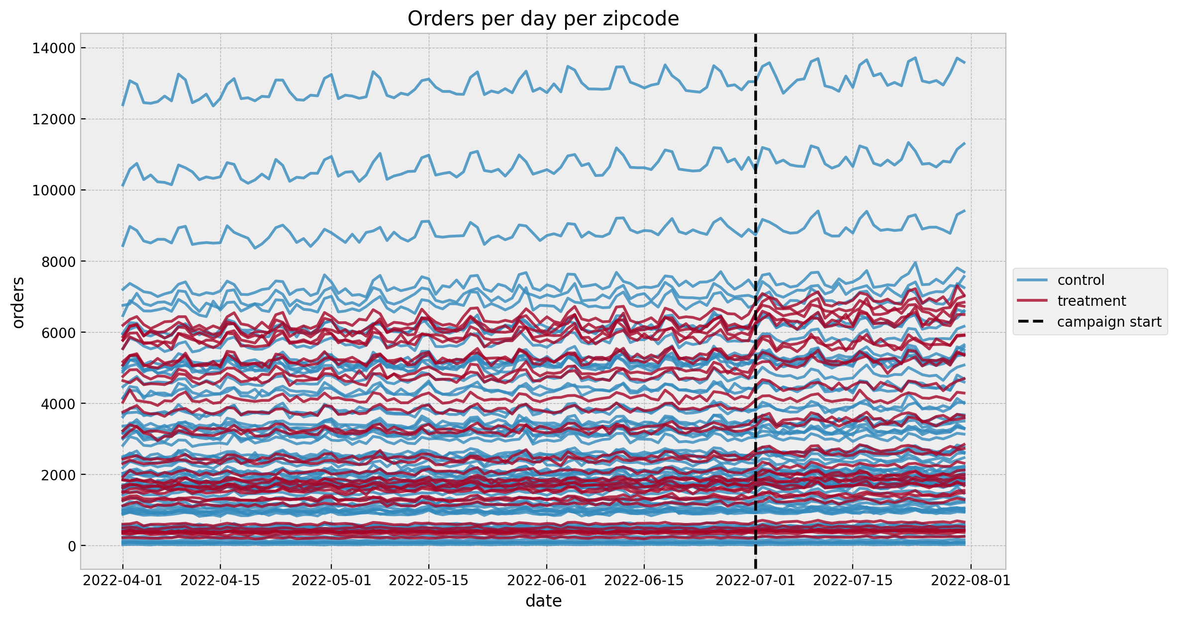
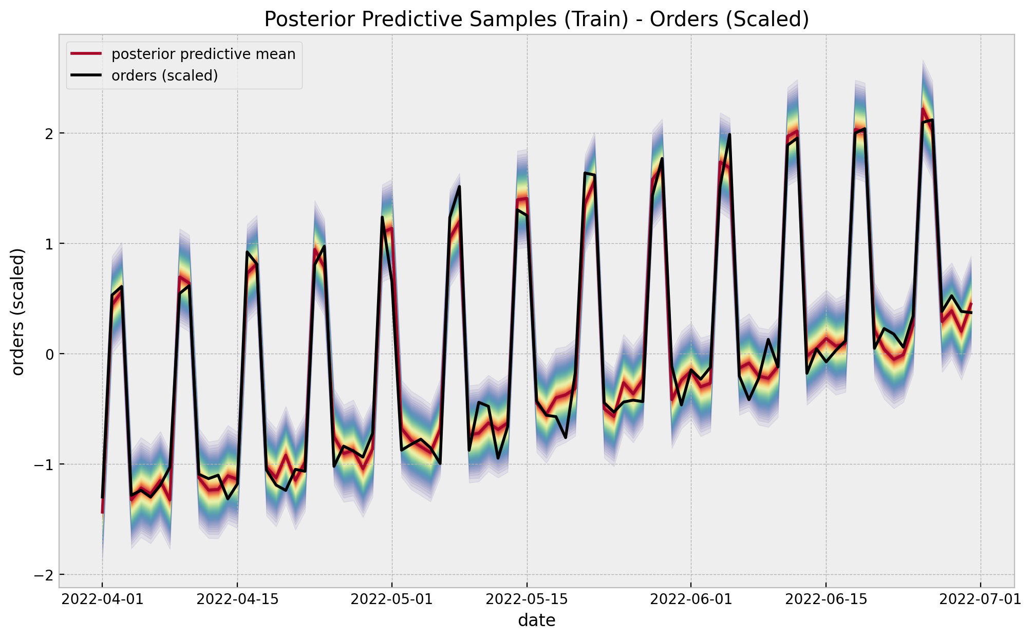
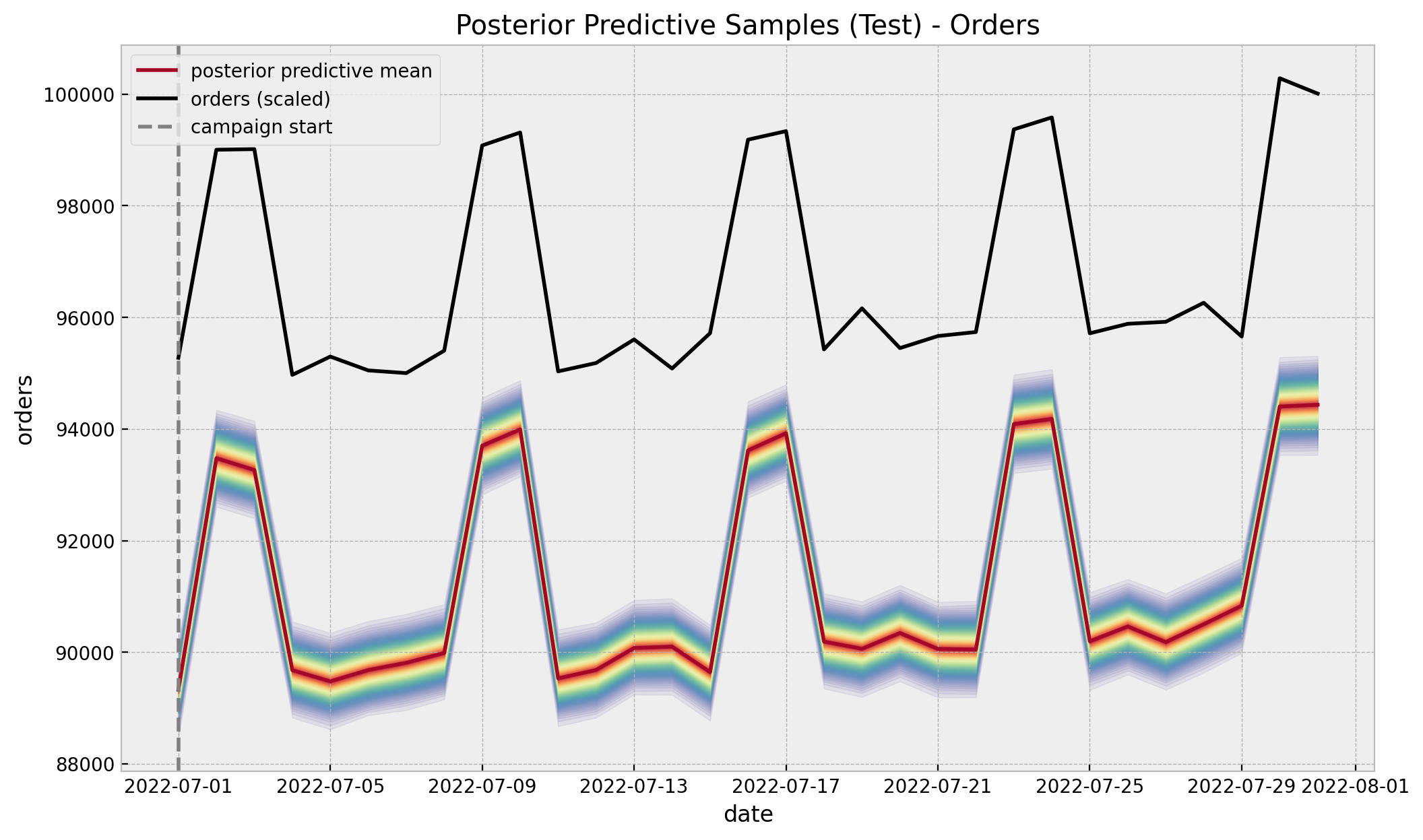
Geo-Experimentation

Time-Based Regression

Linear regression to model the pre-intervention period.

Regression Model in PyMC

with pm.Model() as model:
    # --- Data Containers ---
    model.add_coord(name="date", values=date_train, mutable=True)
    y_control_data = pm.MutableData(
        name="y_control_data", value=y_control_train_scaled, dims="date"
    )
    y_treatment_data = pm.MutableData(
        name="y_treatment_data", value=y_treatment_train_scaled, dims="date"
    )
    # --- Priors ---
    intercept = pm.Normal(name="intercept", mu=0, sigma=1)
    beta = pm.HalfNormal(name="beta", sigma=2)
    sigma = pm.HalfNormal(name="sigma", sigma=2)
    nu = pm.Gamma(name="nu", alpha=20, beta=2)
    # --- Model Parametrization ---
    mu = pm.Deterministic(
      name="mu", var=intercept + beta * y_control_data, dims="date"
    )
    # --- Likelihood ---
    pm.StudentT(
        name="likelihood", mu=mu, nu=nu, sigma=sigma, observed=y_treatment_data, dims="date"
    )

Marketing Measurement

%%{init: {"theme": "white", "themeVariables": {"fontSize": "48px"}, "flowchart":{"htmlLabels":false}}}%%
flowchart LR
  Experimentation("Experimentation") --> MMM("Media Mix Model")
  MMM --> Attribution("Attribution")
  Attribution --> Experimentation

Media Mix Models

• Media Mix Models (MMM) are used by advertisers to measure the effectiveness of their advertising and provide insights for making future budget allocation decisions.

• Media mix models are also used to find the optimal media mix that maximizes the revenue under a budget constraint in the selected time period.

Media Transformations

Carryover (Adstock) & Saturation

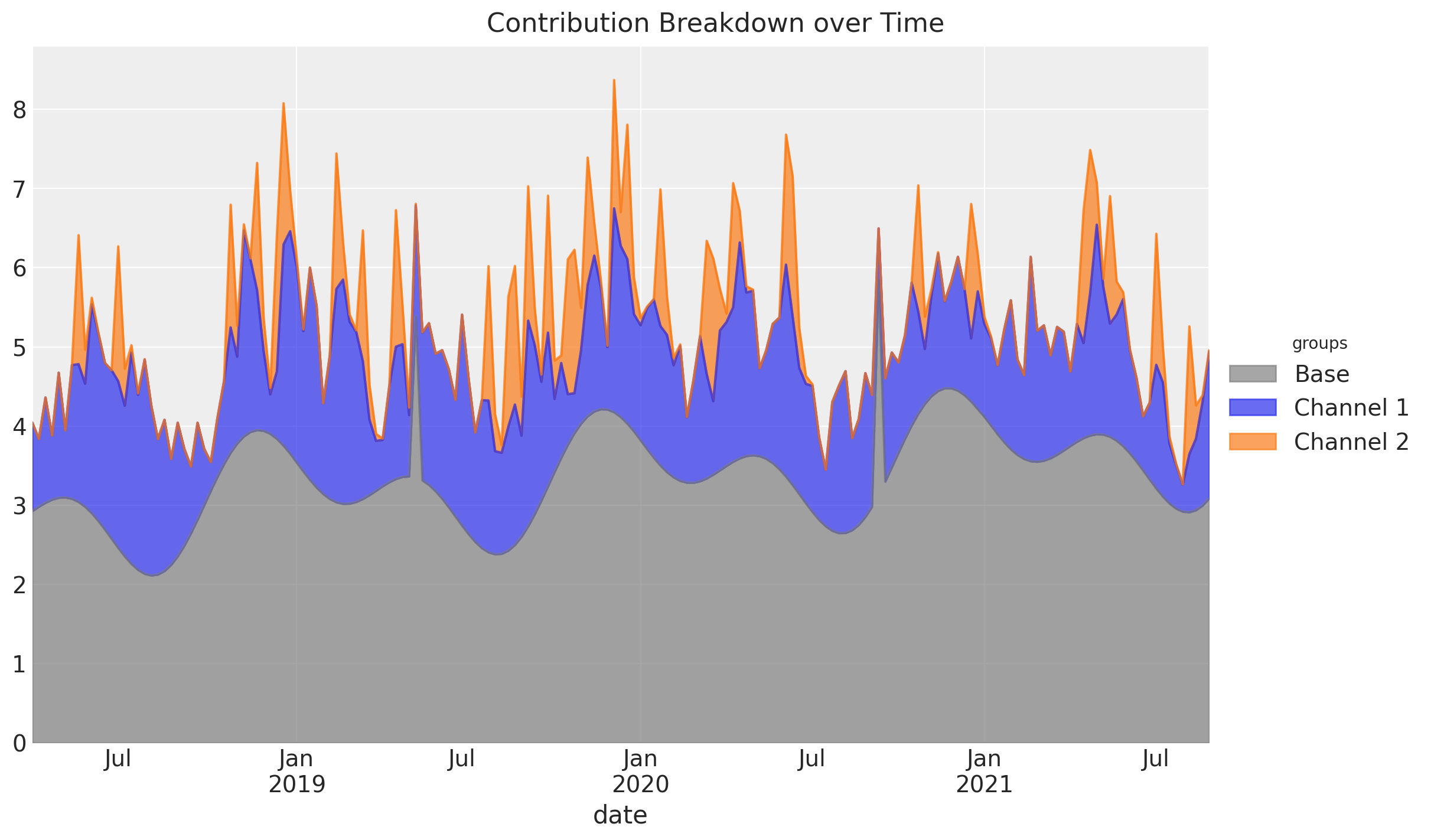
Media Mix Model Target

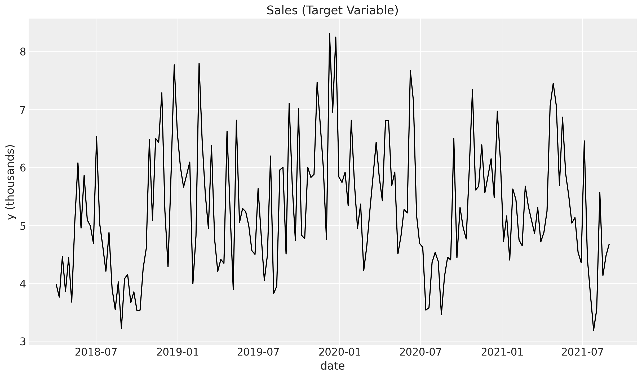
We want to understand the contribution of channels \(x_1\) and \(x_2\) spend into the target variable sales.

MMM Structure

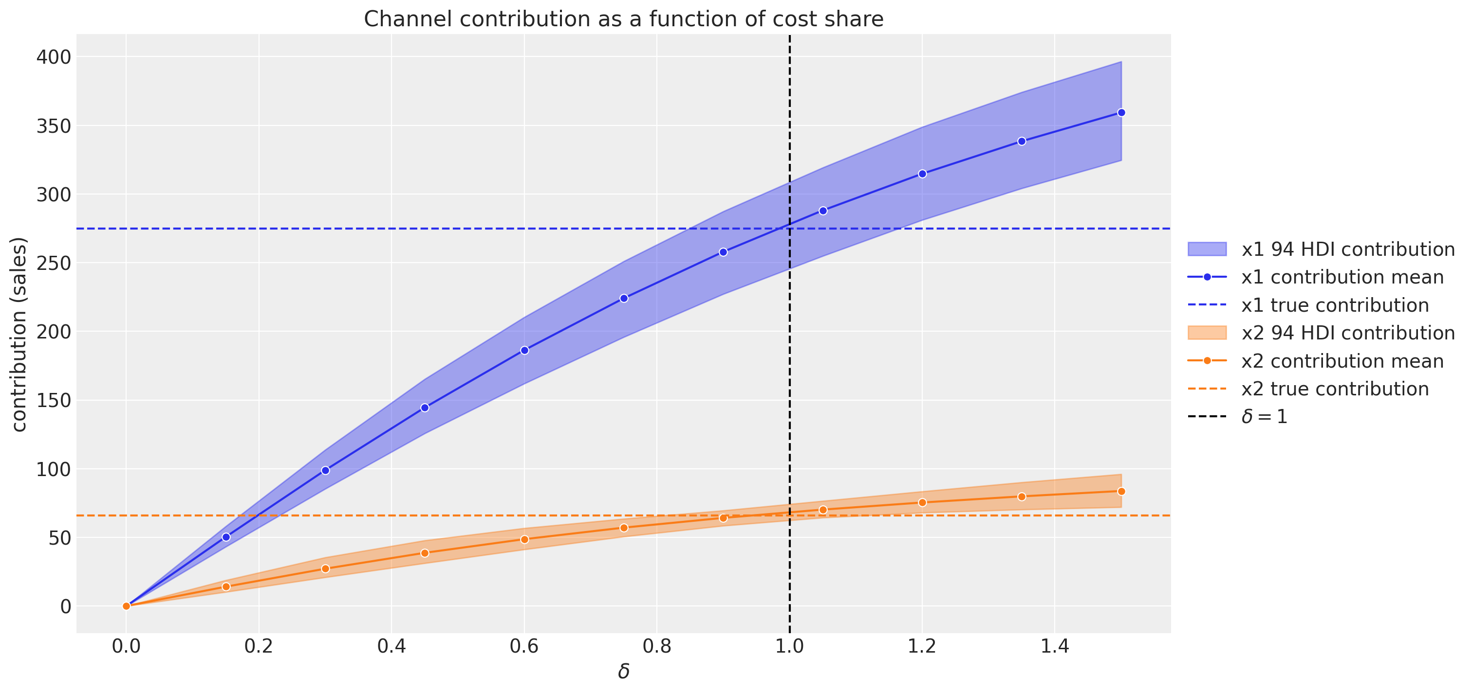
Media Contribution Estimation

Budget Optimization

PyMC-Marketing

Bayesian marketing toolbox in PyMC. Media Mix (MMM), customer lifetime value (CLV), buy-till-you-die (BTYD) models and more.

mmm = DelayedSaturatedMMM(
    data=data,
    target_column="y",
    date_column="date_week",
    channel_columns=["x1", "x2"],
    control_columns=[
        "event_1",
        "event_2",
        "t",
    ],
    adstock_max_lag=8,
    yearly_seasonality=2,
)

Info: www.pymc-marketing.io

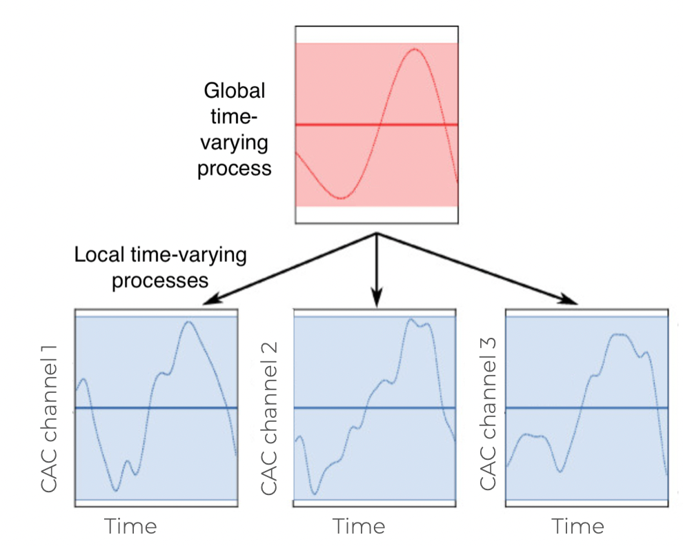
PyMC-Marketing - More MMM Flavours

Very ambitious plans! E.g. Time-varying coefficients through hierarchical Gaussian Processes

Customer Lifetime Value (CLV)

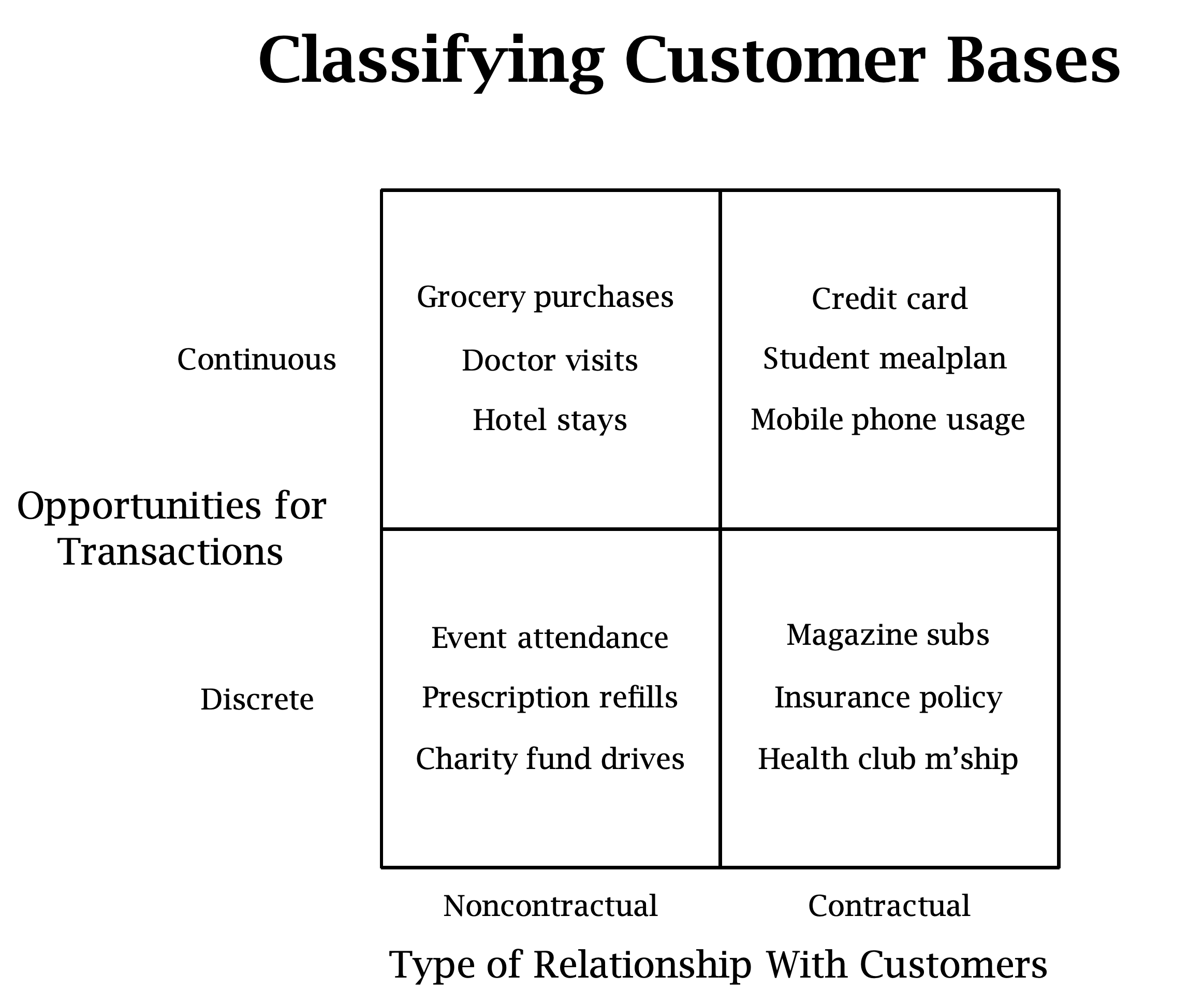
Continuous Non-Contractractual CLV

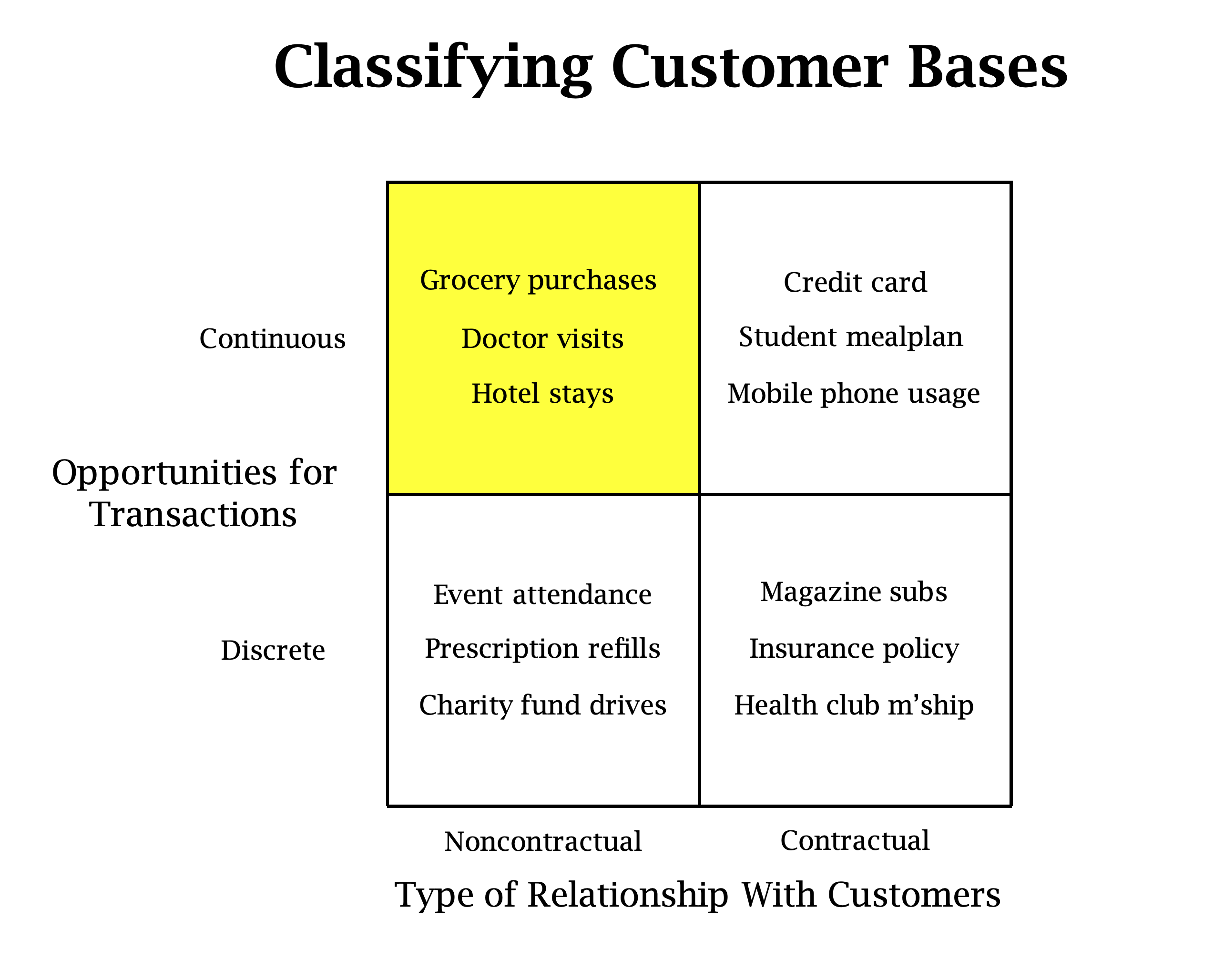
• frequency: Number of repeat purchases the customer has made.

• T: Age of the customer in whatever time units chosen.

• recency: Age of the customer when they made their most recent purchases.

CLV Estimation Strategy

%%{init: {"theme": "dark", "themeVariables": {"fontSize": "48px"}, "flowchart":{"htmlLabels":false}}}%%
flowchart LR
    Recency("Recency") --> BGNBD(["BG/NBD"])
    T("T") --> BGNBD
    Frequency("Frequency") --> BGNBD
    Recency("Recency") --> GammaGamma(["Gamma-Gamma"])
    T --> GammaGamma
    Frequency("Frequency") --> GammaGamma
    MonetaryValue("Monetary Value") --> GammaGamma
    BGNBD --> ProbabilityAlive("Probability Alive")
    BGNBD --> PurchasePrediction("Purchase Prediction")
    GammaGamma --> MonetaryValuePrediction("Monetary Value Prediction")
    PurchasePrediction --> CLV(("CLV"))
    MonetaryValuePrediction --> CLV

    style BGNBD fill:#ff3660
    style GammaGamma fill:#ff3660
    style ProbabilityAlive fill:#1790D0
    style PurchasePrediction fill:#1790D0
    style MonetaryValuePrediction fill:#1790D0
    style CLV fill:#0bb09d

BG/NBD Assumptions

1. While active, the time between transactions is distributed exponentially with transaction rate, i.e.,

   \[f(t_{j}|t_{j-1}; \lambda) = \lambda \exp(-\lambda (t_{j} - t_{j - 1})), \quad t_{j} \geq t_{j - 1} \geq 0\]

2. Heterogeneity in \(\lambda\) follows a gamma distribution with pdf

   \[f(\lambda|r, \alpha) = \frac{\alpha^{r}\lambda^{r - 1}\exp(-\lambda \alpha)}{\Gamma(r)}, \quad \lambda > 0\]

3. After any transaction, a customer becomes inactive with probability \(p\).

4. Heterogeneity in \(p\) follows a beta distribution with pdf

   \[f(p|a, b) = \frac{\Gamma(a + b)}{\Gamma(a) \Gamma(b)} p^{a - 1}(1 - p)^{b - 1}, \quad 0 \leq p \leq 1\]

5. The transaction rate \(\lambda\) and the dropout probability \(p\) vary independently across customers.

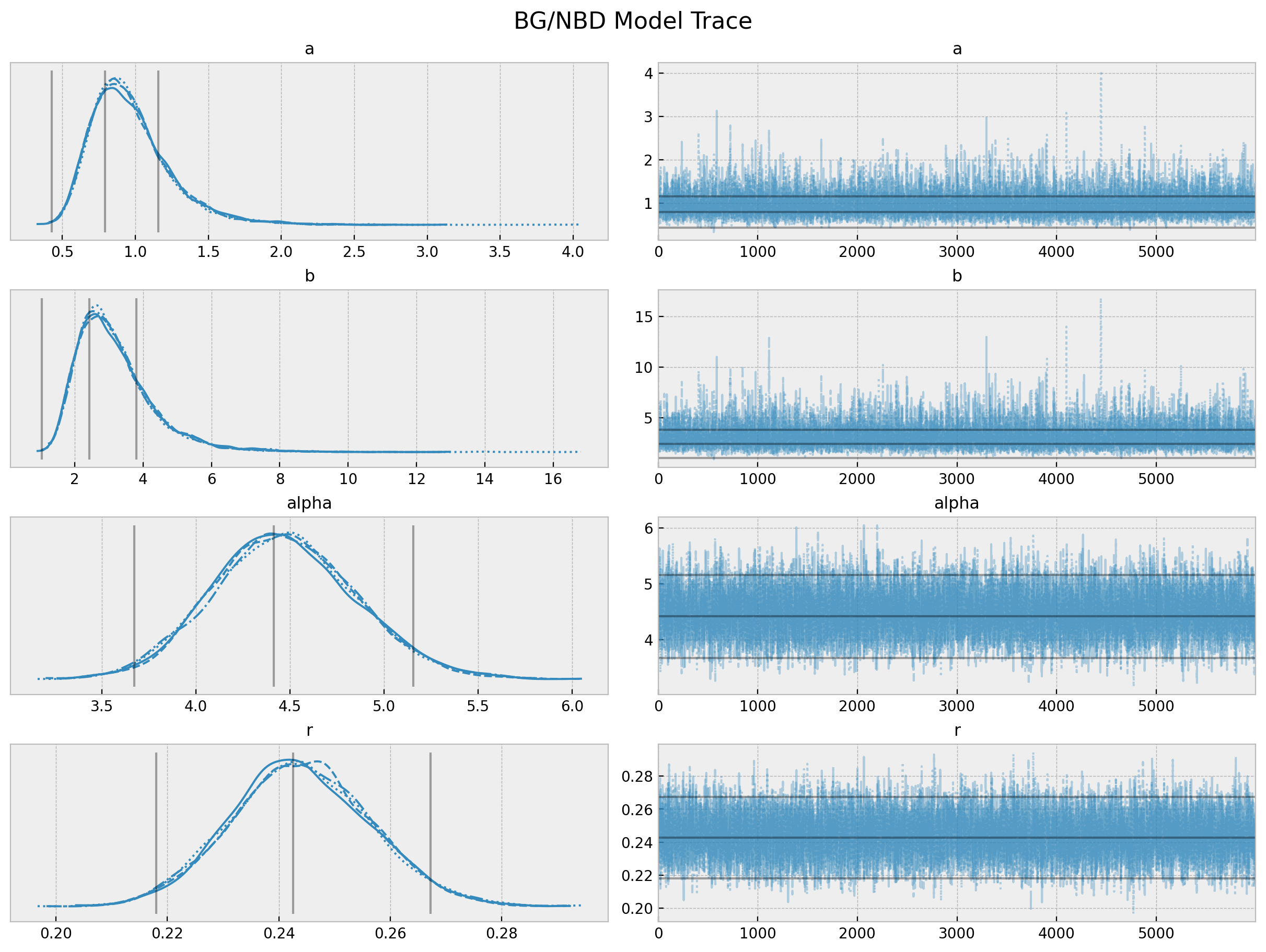
BG/NBD - Parameter Estimation

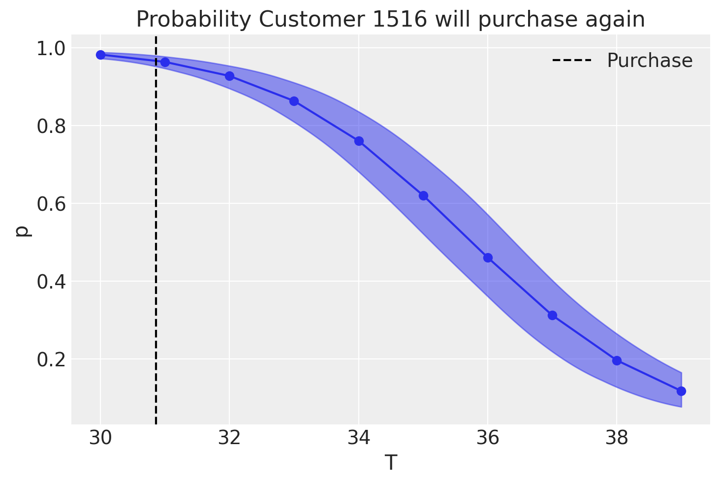
BG/NBD - Probability of Alive

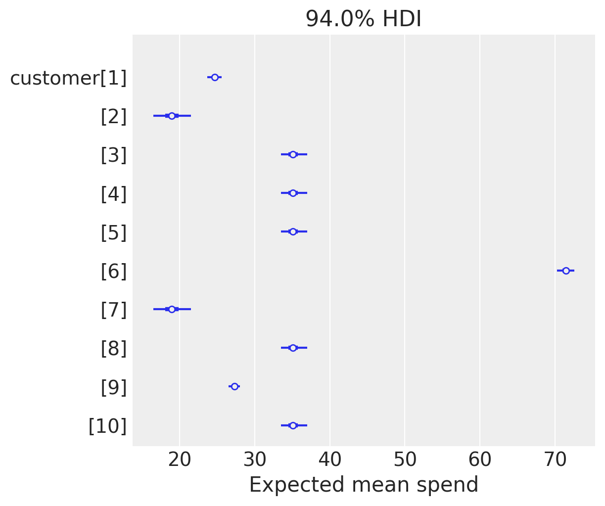
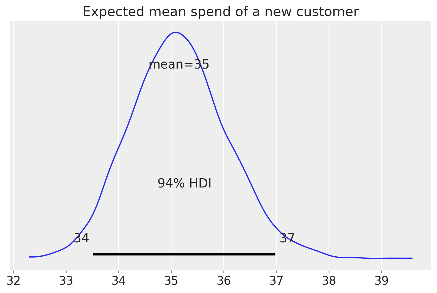
Gamma-Gamma Model

We can estimate the distribution spend for new customers.

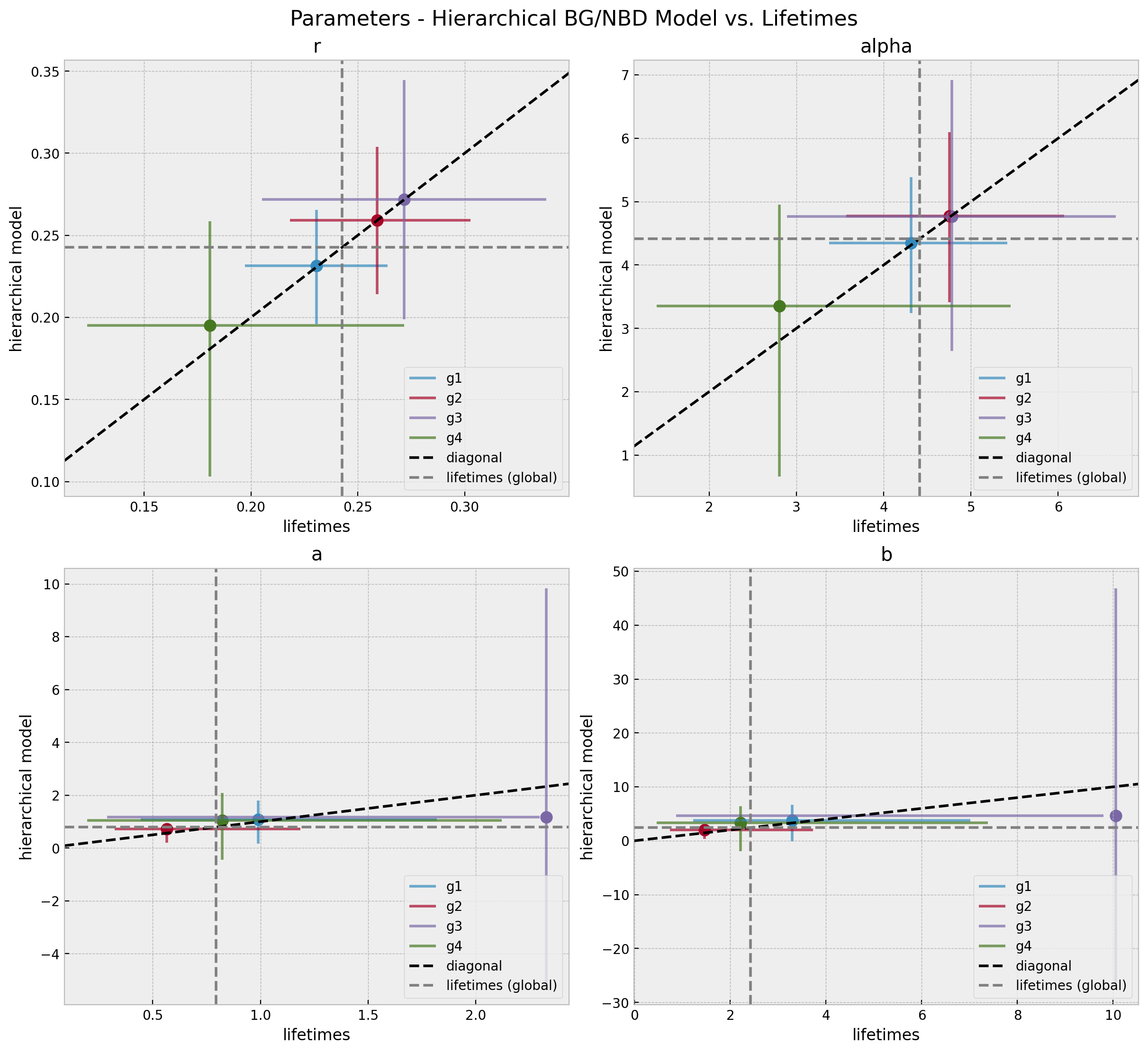
BG/NBD - Hierarchical Models

Causal Inference

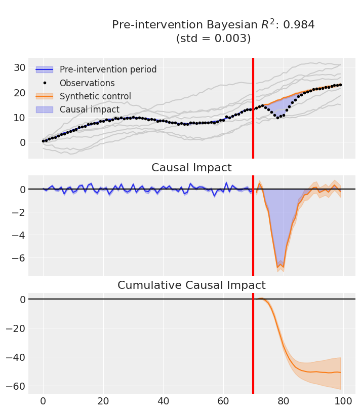
Synthetic Control

Causal Inference

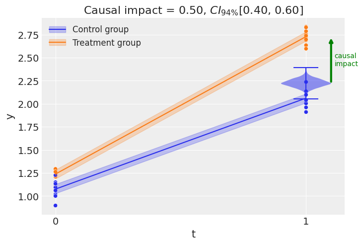
Difference-in-Differences

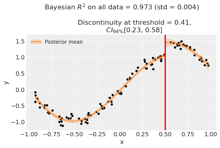
Regression Discontinuity

Instrumental Variables

Cohort Revenue-Retention Modeling

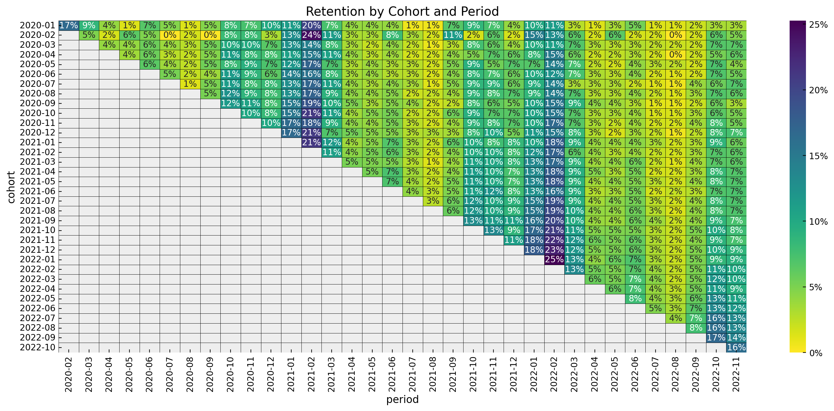
• Cohort Age: Age of the cohort in months.
• Age: Age of the cohort with respect to the observation time.
• Month: Month of the observation time (period).

Retention Component

\[\begin{align*} \textrm{logit}(p) & = \text{BART}(\text{cohort age}, \text{age}, \text{month}) \\ N_{\text{active}} & \sim \text{Binomial}(N_{\text{total}}, p) \end{align*}\]

Revenue Component

\[\begin{align*} \log(\lambda) = \: (& \text{intercept} \\ & + \beta_{\text{cohort age}} \text{cohort age} \\ & + \beta_{\text{age}} \text{age} \\ & + \beta_{\text{cohort age} \times \text{age}} \text{cohort age} \times \text{age}) \\ \text{Revenue} & \sim \text{Gamma}(N_{\text{active}}, \lambda) \end{align*}\]

Cohot Revenue-Retention Model

mu = pmb.BART(name="mu", X=x, Y=train_retention_logit, m=50, dims="obs")

p = pm.Deterministic(name="p", var=pm.math.invlogit(mu), dims="obs")

lam_log = pm.Deterministic(
    name="lam_log",
    var=intercept
    + b_age_scaled * age_scaled
    + b_cohort_age_scaled * cohort_age_scaled
    + b_age_cohort_age_interaction * age_scaled * cohort_age_scaled,
    dims="obs",
)

lam = pm.Deterministic(name="lam", var=pm.math.exp(lam_log), dims="obs")

n_active_users_estimated = pm.Binomial(
    name="n_active_users_estimated",
    n=n_users,
    p=p,
    observed=n_active_users,
    dims="obs",
)

x = pm.Gamma(
    name="revenue_estimated",
    alpha=n_active_users_estimated + eps,
    beta=lam,
    observed=revenue,
    dims="obs",
)

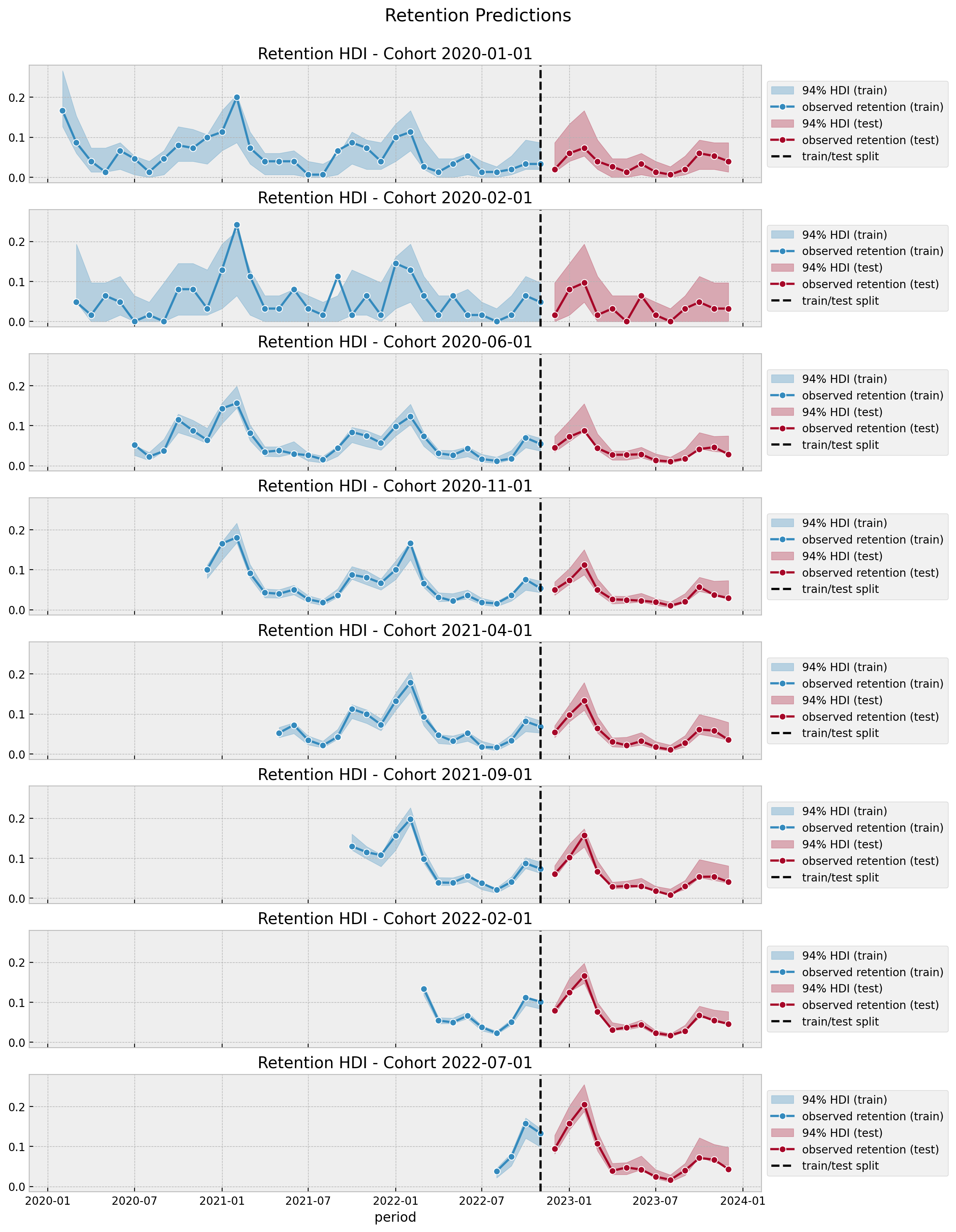
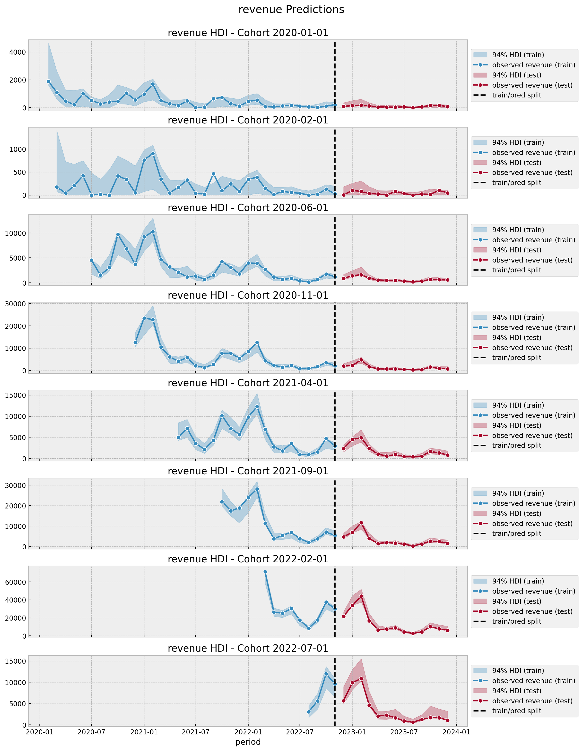
Cohort Revenue-Retention Model

Revenue-Retention - Predictions

References

Media Mix Models

• Bayesian Methods for Media Mix Modeling with Carryover and Shape Effects

• PyMC bayesian model details: Media Effect Estimation with PyMC: Adstock, Saturation & Diminishing Returns

• pymc-marketing: Bayesian marketing toolbox in PyMC. Media Mix (MMM), customer lifetime value (CLV), buy-till-you-die (BTYD) models and more.

• Bayesian Media Mix Models: Modelling changes in marketing effectiveness over time, by PyMC Labs

Customer Lifetime Value

• Probability Models for Customer-Base Analysis

• “Counting Your Customers” the Easy Way: An Alternative to the Pareto/NBD Model

• BG/NBD Model in PyMC

References

Geo-Experimentaton

• Geo-Experimentation via Time-Based Regression in PyMC

• Offline Campaign Analysis Measurement: A journey through causal impact, geo-experimentation and synthetic control

Causal Inference

• CausalPy: A Python package for causal inference in quasi-experimental settings

• Experimentation, Non-Compliance and Instrumental Variables with PyMC

Revenue-Retention Modeling

• A Simple Cohort Retention Analysis in PyMC

• Cohort Retention Analysis with BART

• Cohort Revenue & Retention Analysis: A Bayesian Approach

Thank you!

juanitorduz.github.io

Connect with PyMC Labs

🔗 Learn more about pymc-marketing:

• 🐙 GitHub: https://github.com/pymc-labs/pymc-marketing
• 📝 Documentation: https://www.pymc-marketing.io/en/stable/

🔗 Connecting with PyMC Labs:

• 👥 LinkedIn: https://www.linkedin.com/company/pymc-labs/
• 🐦 Twitter: https://twitter.com/pymc_labs
• 🎥 YouTube: https://www.youtube.com/PyMCLabs
• 🤝 Meetup: https://www.meetup.com/pymc-labs-online-meetup/