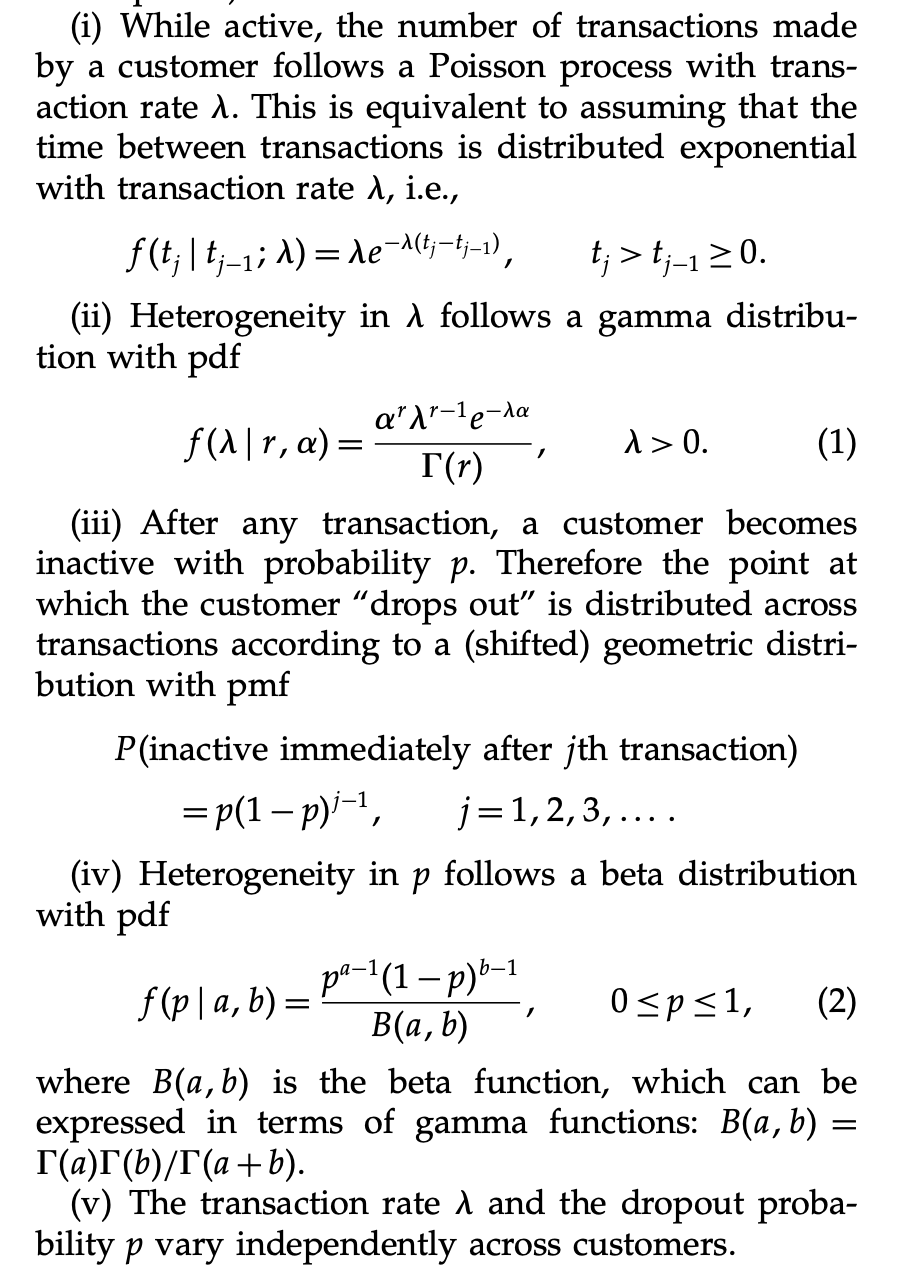
In this notebook we show how to port the BG/NBD model from the the lifetimes (developed mainly by Cameron Davidson-Pilon) package to pymc. The BG/NBD model, introduced in the seminal paper “Counting Your Customers” the Easy Way: An Alternative to the Pareto/NBD Model by Peter S. Fader, Bruce G. S. Hardie and Ka Lok Lee in 2005, is used to
predict future purchasing patterns, which can then serve as an input into “lifetime value” calculations, in the “non-contractual” setting (i.e., where the opportunities for transactions are continuous and the time at which customers become inactive is unobserved).
Why to port the BG/NBD model to pymc?
- The
lifetimespackage is currently in “maintenance-mode”, so we do not expect it to be further developed. In addition, I am not aware of other python implementation (the R community has more options available) - This current implementation does not allow for time-invariant external covariates even though is an easy extension an shown in the paper Incorporating Time-Invariant Covariates into the Pareto/NBD and BG/NBD Models by Peter S. Fader and Bruce G. S. Hardie. There is actually an open PR to att his feature into the
lifetimespackage, but it is highly unlikely to be merged. Hence, as in practice time-invariant covariates could further segment user purchase patterns, writing this model explicitly can allow for more flexibility. - We can take advantage of the powerful bayesian machinery to have better uncertainty estimation and the possibility to use extend the base BG/NBD model to more complex ones, e.g. hierarchical models.
Remark: The content of this post was presented at the Berlin Bayesians MeetUp in September 2022. Here you can find the slides.
Prepare Notebook
mport arviz as az
import matplotlib.pyplot as plt
import numpy as np
import pandas as pd
import pymc as pm
import pytensor.tensor as pt
import seaborn as sns

from lifetimes import BetaGeoFitter


from lifetimes.datasets import load_cdnow_summary
from scipy.special import expit, hyp2f1


az.style.use("arviz-darkgrid")
plt.rcParams["figure.figsize"] = [12, 7]
plt.rcParams["figure.dpi"] = 100
plt.rcParams["figure.facecolor"] = "white"

seed = sum(map(ord, "juanitorduz"))
rng = np.random.default_rng(seed)

%load_ext autoreload
%autoreload 2
%config InlineBackend.figure_format = "retina"
Load Data
We are going to use an existing data set from the lifetimes package documentation, see here.
data_df = load_cdnow_summary(index_col=[0])

n_obs = data_df.shape[0]

data_df.info()
<class 'pandas.core.frame.DataFrame'>
Int64Index: 2357 entries, 1 to 2357
Data columns (total 3 columns):
# Column Non-Null Count Dtype
--- ------ -------------- -----
0 frequency 2357 non-null int64
1 recency 2357 non-null float64
2 T 2357 non-null float64
dtypes: float64(2), int64(1)
memory usage: 73.7 KBFrom the package’s documentation:
frequency: Number of repeat purchases the customer has made. More precisely, It’s the count of time periods the customer had a purchase in.T: Age of the customer in whatever time units chosen (weekly, in the above dataset). This is equal to the duration between a customer’s first purchase and the end of the period under study.recency: Age of the customer when they made their most recent purchases. This is equal to the duration between a customer’s first purchase and their latest purchase.
data_df.head(10)| frequency | recency | T | |
|---|---|---|---|
| ID | |||
| 1 | 2 | 30.43 | 38.86 |
| 2 | 1 | 1.71 | 38.86 |
| 3 | 0 | 0.00 | 38.86 |
| 4 | 0 | 0.00 | 38.86 |
| 5 | 0 | 0.00 | 38.86 |
| 6 | 7 | 29.43 | 38.86 |
| 7 | 1 | 5.00 | 38.86 |
| 8 | 0 | 0.00 | 38.86 |
| 9 | 2 | 35.71 | 38.86 |
| 10 | 0 | 0.00 | 38.86 |
Let us extract the data as arrays and recover the notation from the original papers.
n = data_df.shape[0]
x = data_df["frequency"].to_numpy()
t_x = data_df["recency"].to_numpy()
T = data_df["T"].to_numpy()

# convenient indicator function
int_vec = np.vectorize(int)
x_zero = int_vec(x > 0)
BG/NBD Model (Lifetimes)
We do not want to give a detailed description of the model, so we will just show the notation. Please refer to the original papers for more details, e.g. “Counting Your Customers” the Easy Way: An Alternative to the Pareto/NBD Model.
We now use the lifetimes object BetaGeoFitter to estimate the model parameters via maximum likelihood estimation.
# fit BG/NBD model
bgf = BetaGeoFitter()
bgf.fit(frequency=x, recency=t_x, T=T)

bgf.summary| coef | se(coef) | lower 95% bound | upper 95% bound | |
|---|---|---|---|---|
| r | 0.242593 | 0.012557 | 0.217981 | 0.267205 |
| alpha | 4.413532 | 0.378221 | 3.672218 | 5.154846 |
| a | 0.792886 | 0.185719 | 0.428877 | 1.156895 |
| b | 2.425752 | 0.705345 | 1.043276 | 3.808229 |
Note that the models provide confidence intervals for the estimated parameters. These are estimated using by using the Hessian to calculate the variance matrix, see Standard error from Hessian matrix when likelihood is used (rather than Ln L).
Full Bayesian Model
A nice pymc implementation of the full bayesian model can be found in the blog post Implementing Fader Hardie (2005) in pymc3 by Sid Ravinutala. In this post, the author uses the complete likelihood function (Equation (3) in “Counting Your Customers” the Easy Way: An Alternative to the Pareto/NBD Model):
\[ L(\lambda, p | X=x, T) = (1 - p)^{x}\lambda^{x}e^{-\lambda T} + \delta_{X > 0}p(1 - p)^{x - 1}\lambda^x e^{-\lambda t_x} \]
Here is the model in pymc:
with pm.Model() as model_full:
    # hyper priors for the Gamma params
    a = pm.HalfNormal(name="a", sigma=10)
    b = pm.HalfNormal(name="b", sigma=10)

    # hyper priors for the Beta params
    alpha = pm.HalfNormal(name="alpha", sigma=10)
    r = pm.HalfNormal(name="r", sigma=10)

    lam = pm.Gamma(name="lam", alpha=r, beta=alpha, shape=n)
    p = pm.Beta(name="p", alpha=a, beta=b, shape=n)

    def logp(x, t_x, T, x_zero):
        log_term_a = x * pt.log(1 - p) + x * pt.log(lam) - t_x * lam
        term_b_1 = -lam * (T - t_x)
        term_b_2 = pt.log(p) - pt.log(1 - p)
        log_term_b = pm.math.switch(
            x_zero, pm.math.logaddexp(term_b_1, term_b_2), term_b_1
        )

        return pt.sum(log_term_a) + pt.sum(log_term_b)

    likelihood = pm.Potential(
        name="likelihood",
        var=logp(x=x, t_x=t_x, T=T, x_zero=x_zero),
    )

pm.model_to_graphviz(model=model_full)
with model_full:
    trace_full = pm.sample(
        tune=2_000,
        draws=4_000,
        chains=4,
        target_accept=0.95,
        nuts_sampler="numpyro",
    )
This model takes a while to run and the results coincide with the ones from obtained using lifetimes.
axes = az.plot_trace(
    data=trace_full,
    var_names=["a", "b", "alpha", "r"],
    lines=[
        (k, {}, [v.to_numpy()])
        for k, v in bgf.summary[
            ["coef", "lower 95% bound", "upper 95% bound"]
        ].T.items()
    ],
    compact=True,
    backend_kwargs={"figsize": (12, 9), "layout": "constrained"},
)
fig = axes[0][0].get_figure()
fig.suptitle("Full BG/NBD Model Trace", fontsize=16, fontweight="bold");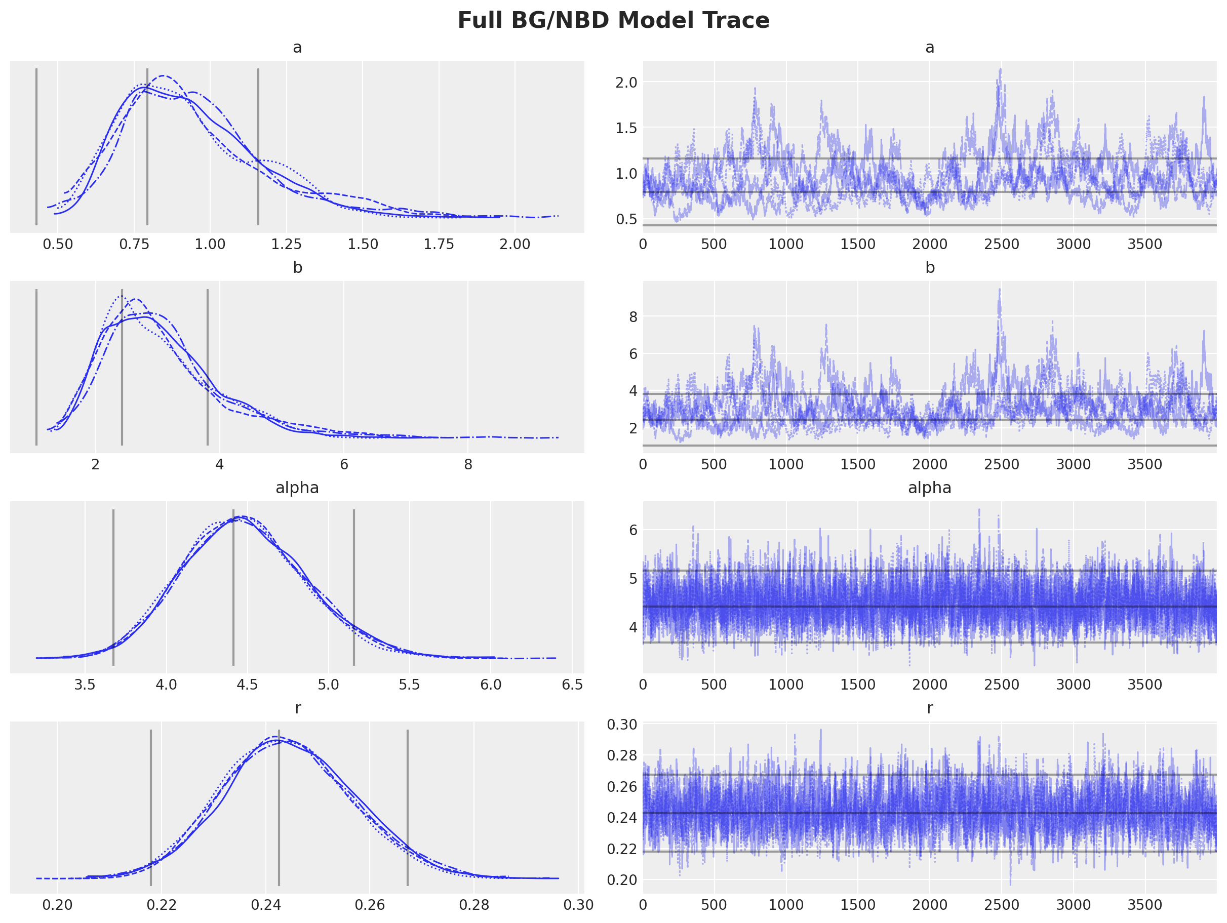
axes = az.plot_pair(data=trace_full, var_names=["a", "b", "alpha", "r"], figsize=(12, 12))
fig = axes[0][0].get_figure()
fig.suptitle("Full BG/NBD Model Parameters Pairplot", fontsize=16, fontweight="bold");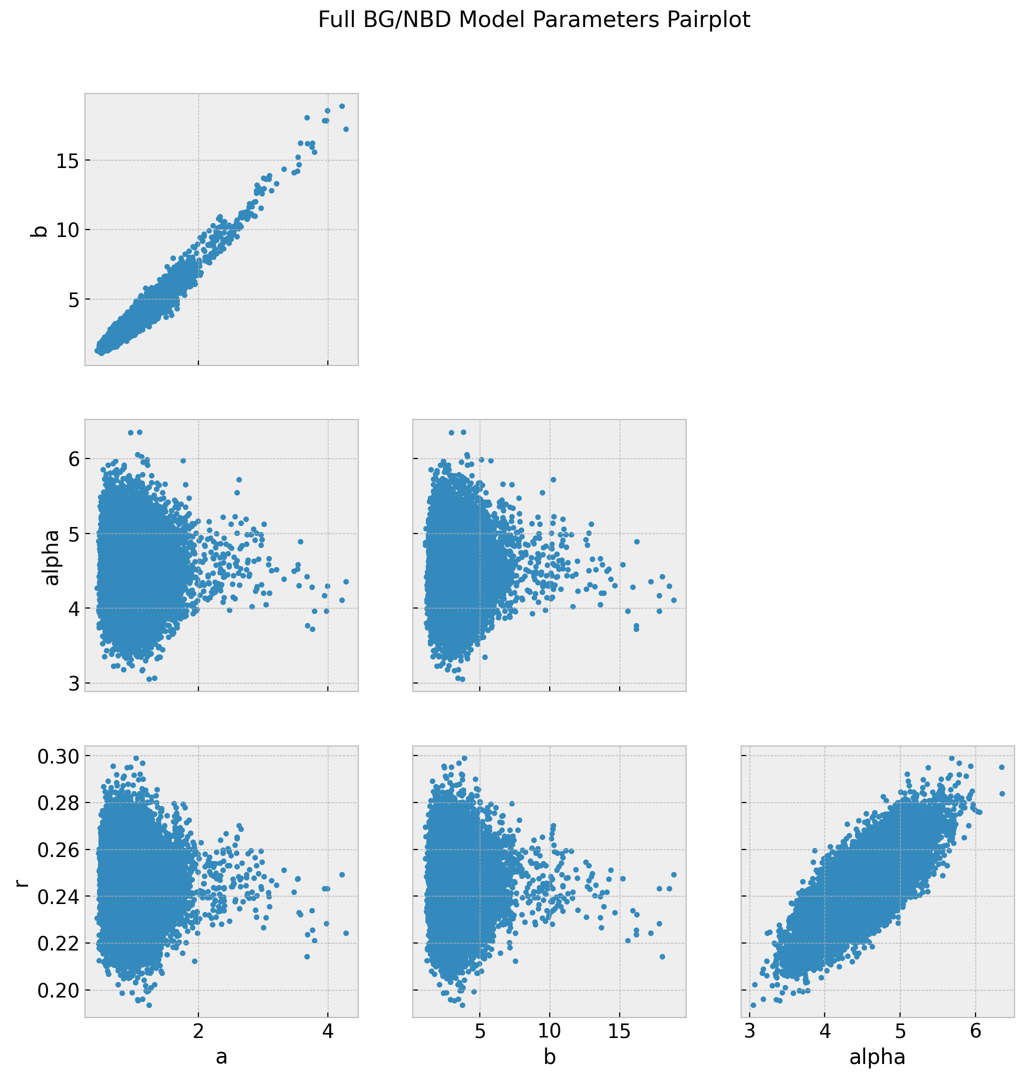
The chains for a and b do not look so good. We actually see from the pairplot that these parameters highly correlated. See the r_hat values below.
az.summary(data=trace_full, var_names=["a", "b", "alpha", "r"])| mean | sd | hdi_3% | hdi_97% | mcse_mean | mcse_sd | ess_bulk | ess_tail | r_hat | |
|---|---|---|---|---|---|---|---|---|---|
| a | 0.949 | 0.284 | 0.513 | 1.399 | 0.026 | 0.018 | 108.0 | 214.0 | 1.03 |
| b | 3.095 | 1.202 | 1.437 | 5.053 | 0.103 | 0.073 | 118.0 | 287.0 | 1.02 |
| alpha | 4.467 | 0.384 | 3.757 | 5.196 | 0.008 | 0.005 | 2608.0 | 6504.0 | 1.00 |
| r | 0.244 | 0.013 | 0.219 | 0.267 | 0.000 | 0.000 | 1913.0 | 4427.0 | 1.00 |
Bayesian Model: Randomly Chosen Individual
One drawback (computationally) of the model_full is that we have \(\lambda\) and \(p\) parameters per user. This does not scale that easily. That is why in practice one usually takes the expectation over \(\lambda\) and \(p\) to study a randomly chosen individual. One can compute this expectation analytically, see Section \(5\) in “Counting Your Customers” the Easy Way: An Alternative to the Pareto/NBD Model for the mathematical details. What is important to remark is this the end expression for the log-likelihood is relatively easy to write. Actually, the authors of the paper have a document which describes how to estimate the corresponding parameters in Excel, see Implementing the BG/NBD Model for Customer Base Analysis in Excel. The resulting expression for the likelihood function is:
\[ L(a, b, \alpha, r|X=x, t_x, T) = A_{1}A_{2}(A_{3} + \delta_{x>0}A_4) \]
where
\[\begin{align*} A_{1} & = \frac{\Gamma(r + x)\alpha^{{r}}}{\Gamma(x)} \\ A_{2} & = \frac{\Gamma(a + b)\Gamma(b + x)}{\Gamma(b)\Gamma(a + b + x)} \\ A_{3} & = \left(\frac{1}{\alpha + T}\right)^{r+x} \\ A_{4} & = \left(\frac{a}{b + x - 1}\right)\left(\frac{1}{\alpha + t_x}\right)^{r + x} \end{align*}\]
Computing the \(\log (L(a, b, \alpha, r|X=x, t_x, T))\) is straight forward from these explicit expressions \(a_{i} := \log(A_{i})\). Note however that one has to be careful with the \(a_{4} := \log(A_4)\) term since we need to ensure that \(b + x - 1 >0\) (otherwise should be zero). Fortunately, we can simple re-factor the log-likelihood method code of th lifetimes’s BetaGeoFitter class from numpy to pytensor (see lifetimes.BetaGeoFitter._negative_log_likelihood).
with pm.Model() as model:
    a = pm.HalfNormal(name="a", sigma=10)
    b = pm.HalfNormal(name="b", sigma=10)

    alpha = pm.HalfNormal(name="alpha", sigma=10)
    r = pm.HalfNormal(name="r", sigma=10)

    def logp(x, t_x, T, x_zero):
        a1 = pt.gammaln(r + x) - pt.gammaln(r) + r * pt.log(alpha)
        a2 = (
            pt.gammaln(a + b)
            + pt.gammaln(b + x)
            - pt.gammaln(b)
            - pt.gammaln(a + b + x)
        )
        a3 = -(r + x) * pt.log(alpha + T)
        a4 = (
            pt.log(a) - pt.log(b + pt.maximum(x, 1) - 1) - (r + x) * pt.log(t_x + alpha)
        )
        max_a3_a4 = pt.maximum(a3, a4)
        ll_1 = a1 + a2
        ll_2 = (
            pt.log(
                pt.exp(a3 - max_a3_a4)
                + pt.exp(a4 - max_a3_a4) * pm.math.switch(x_zero, 1, 0)
            )
            + max_a3_a4
        )
        return pt.sum(ll_1 + ll_2)

    likelihood = pm.Potential(
        name="likelihood",
        var=logp(x=x, t_x=t_x, T=T, x_zero=x_zero),
    )

pm.model_to_graphviz(model=model)
Let us compute the posterior distributions:
with model:
trace = pm.sample(
tune=2_000,
draws=4_000,
chains=4,
target_accept=0.95,
nuts_sampler="numpyro",
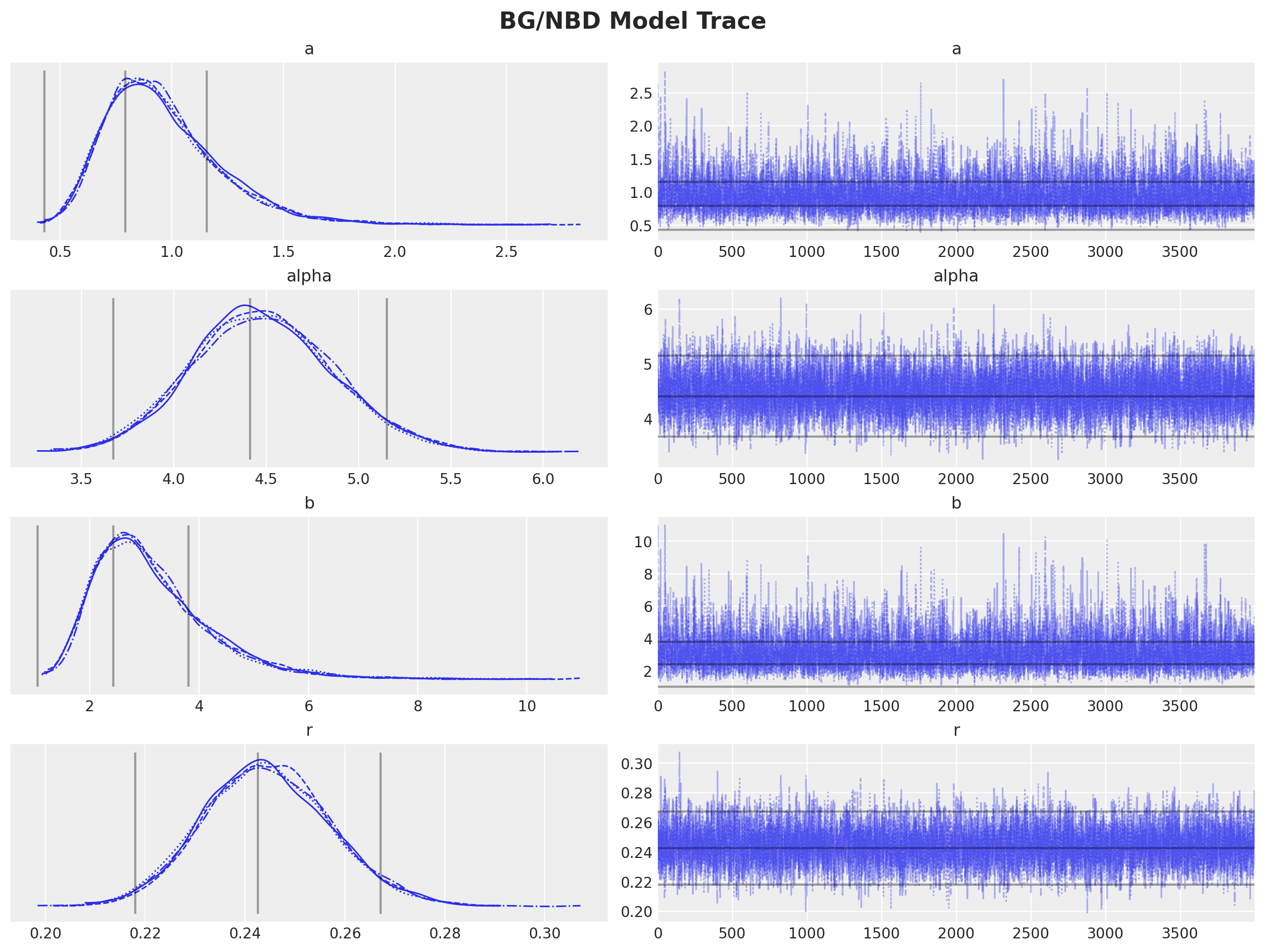
)This model is much faster to train! We can now take a look at the traces, pairplots and summary statistics.
axes = az.plot_trace(
    data=trace,
    lines=[
        (k, {}, [v.to_numpy()])
        for k, v in bgf.summary[
            ["coef", "lower 95% bound", "upper 95% bound"]
        ].T.items()
    ],
    compact=True,
    backend_kwargs={"figsize": (12, 9), "layout": "constrained"},
)
fig = axes[0][0].get_figure()
fig.suptitle("BG/NBD Model Trace", fontsize=16, fontweight="bold");
axes = az.plot_pair(data=trace, figsize=(12, 12))
fig = axes[0][0].get_figure()
ig.suptitle("BG/NBD Model Parameters Pairplot", fontsize=16, fontweight="bold");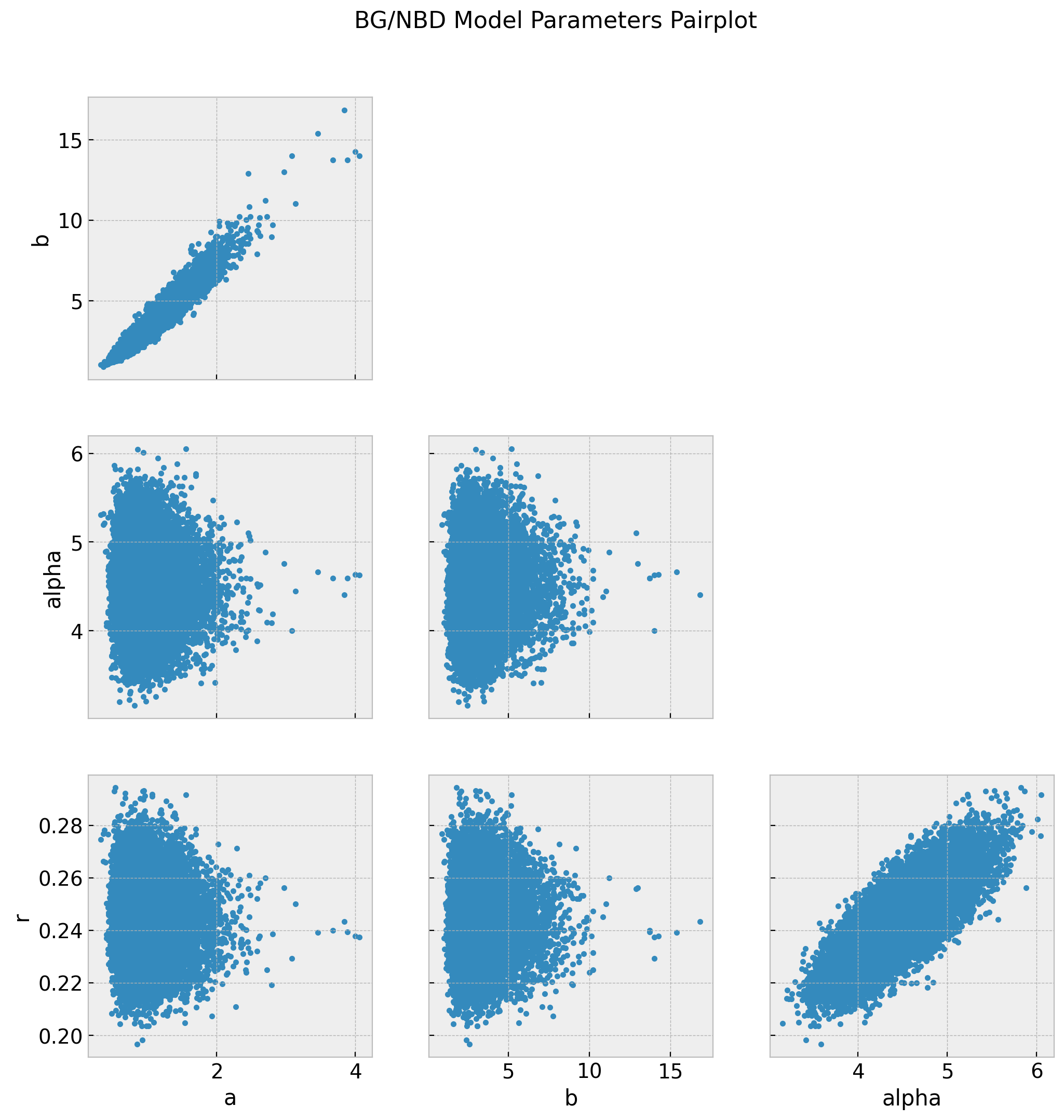
az.summary(data=trace)| mean | sd | hdi_3% | hdi_97% | mcse_mean | mcse_sd | ess_bulk | ess_tail | r_hat | |
|---|---|---|---|---|---|---|---|---|---|
| a | 0.969 | 0.279 | 0.541 | 1.490 | 0.003 | 0.002 | 9063.0 | 9408.0 | 1.0 |
| b | 3.170 | 1.150 | 1.423 | 5.242 | 0.013 | 0.010 | 9134.0 | 9060.0 | 1.0 |
| alpha | 4.472 | 0.382 | 3.757 | 5.184 | 0.004 | 0.003 | 9292.0 | 10149.0 | 1.0 |
| r | 0.244 | 0.012 | 0.220 | 0.267 | 0.000 | 0.000 | 9521.0 | 11044.0 | 1.0 |
The summary statistics look overall good. In particular the chains values for a and b look better than the model_full.
Probability of being alive
Now that we have posterior samples for the model parameters we can easily compute quantities of interest. For example, let us compute the conditional probability of being alive, see the note Computing P(alive) Using
the BG/NBD Model. Again, we can simply port the corresponding method from lifetimes.BetaGeoFitter.conditional_probability_alive.
# See https://docs.pymc.io/en/stable/pymc-examples/examples/time_series/Air_passengers-Prophet_with_Bayesian_workflow.html
def _sample(array, n_samples):
    """Little utility function, sample n_samples with replacement."""
    idx = rng.choice(np.arange(len(array)), n_samples, replace=True)
    return array[idx]


def conditional_probability_alive(trace, x, t_x, T):
    n_vals = x.shape[0]

    a = _sample(array=trace.posterior["a"].to_numpy(), n_samples=n_vals)
    b = _sample(array=trace.posterior["b"].to_numpy(), n_samples=n_vals)
    alpha = _sample(array=trace.posterior["alpha"].to_numpy(), n_samples=n_vals)
    r = _sample(array=trace.posterior["r"].to_numpy(), n_samples=n_vals)

    log_div = (r + x[..., None]) * np.log(
        (alpha + T[..., None]) / (alpha + t_x[..., None])
    ) + np.log(a / (b + np.maximum(x[..., None], 1) - 1))
    return np.where(x[..., None] == 0, 1.0, expit(-log_div))


p_alive_sample = conditional_probability_alive(trace, x, t_x, T)
We compute these probabilities directly from the BetaGeoFitter object directly so that we could compare the results.
p_alive = bgf.conditional_probability_alive(x, t_x, T)We can simply plot some example predictions:
def plot_conditional_probability_alive(p_alive_sample, p_alive, idx, ax):
    sns.kdeplot(x=p_alive_sample[idx], color="C0", fill=True, ax=ax)
    ax.axvline(x=p_alive[idx], color="C1", linestyle="--")
    ax.set(title=f"idx={idx}")
    return ax


fig, axes = plt.subplots(nrows=3, ncols=3, figsize=(9, 9), layout="constrained")
for idx, ax in enumerate(axes.flatten()):
    plot_conditional_probability_alive(p_alive_sample, p_alive, idx, ax)

fig.suptitle("Conditional Probability Alive", fontsize=16, fontweight="bold");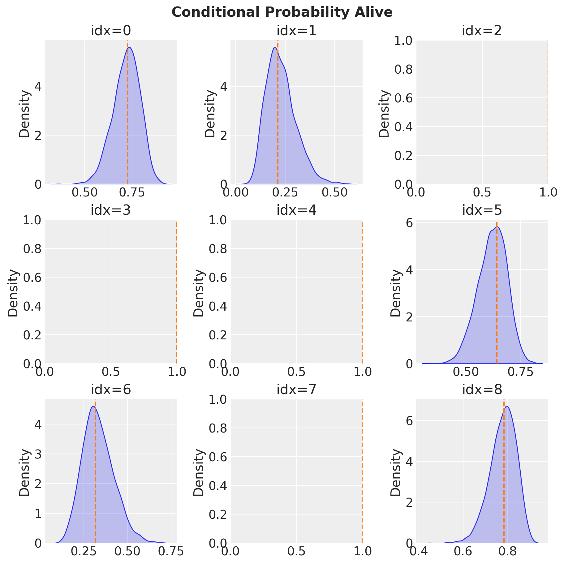
The plots without density correspond to users with probability of being active of \(1.0\). Note for example that for idx=2 we have:
idx = 2
# probability estimation lifetimes model
p_alive[idx]
1.0
# posterior samples
np.unique(p_alive_sample[idx])array([1.])
Hence, the bayesian model also captures the case when the user is certainly alive (because did a very recent purchase).
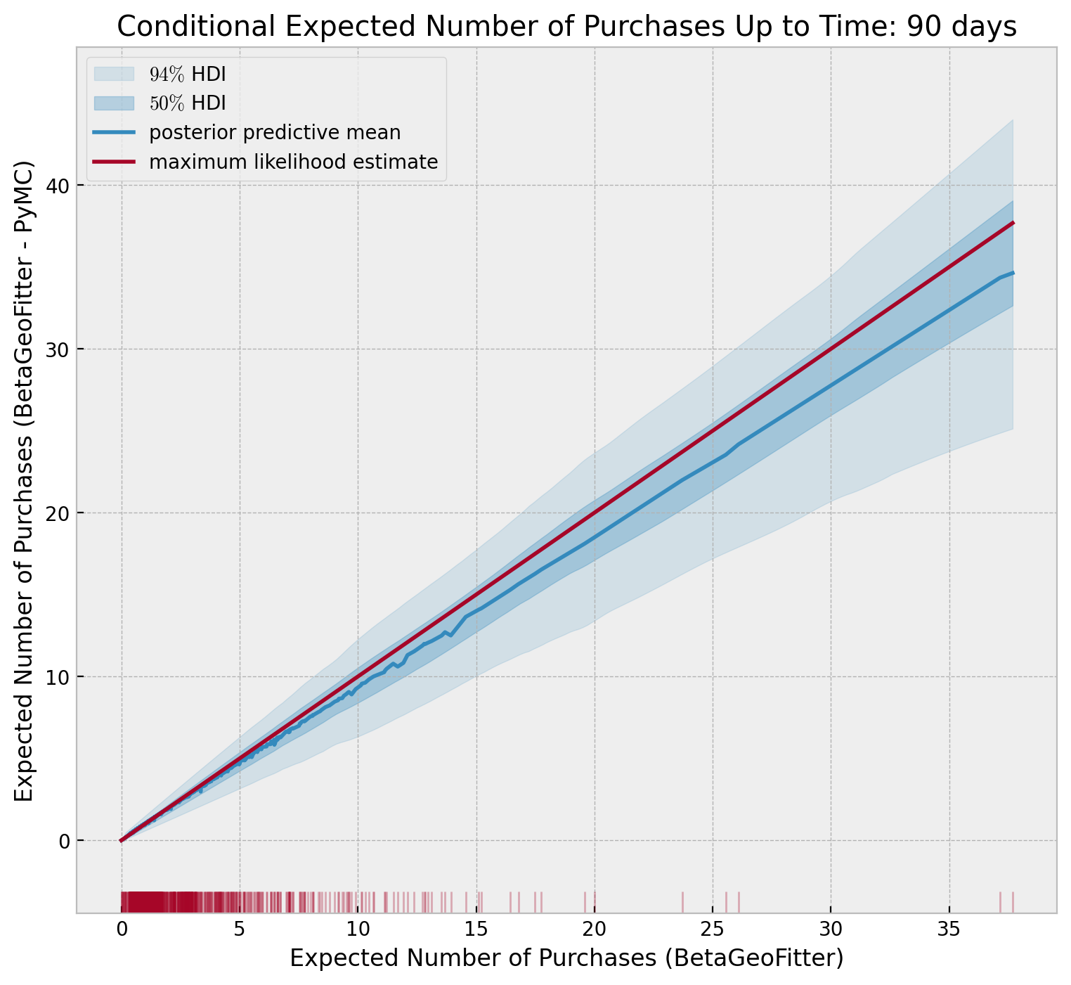
Predicting the number of future transactions
We can do something similar for the expected number of future transactions using the analytical expression implemented in the method lifetimes.BetaGeoFitter. conditional_expected_number_of_purchases_up_to_time.
def conditional_expected_number_of_purchases_up_to_time(t, trace, x, t_x, T):
    n_vals = x.shape[0]
    a = _sample(array=trace.posterior["a"].to_numpy(), n_samples=n_vals)
    b = _sample(array=trace.posterior["b"].to_numpy(), n_samples=n_vals)
    alpha = _sample(array=trace.posterior["alpha"].to_numpy(), n_samples=n_vals)
    r = _sample(array=trace.posterior["r"].to_numpy(), n_samples=n_vals)

    _a = r + x[..., None]
    _b = b + x[..., None]
    _c = a + b + x[..., None] - 1
    _z = t / (alpha + T[..., None] + t)
    ln_hyp_term = np.log(hyp2f1(_a, _b, _c, _z))

    ln_hyp_term_alt = np.log(hyp2f1(_c - _a, _c - _b, _c, _z)) + (
        _c - _a - _b
    ) * np.log(1 - _z)
    ln_hyp_term = np.where(np.isinf(ln_hyp_term), ln_hyp_term_alt, ln_hyp_term)
    first_term = (a + b + x[..., None] - 1) / (a - 1)
    second_term = 1 - np.exp(
        ln_hyp_term
        + (r + x[..., None])
        * np.log((alpha + T[..., None]) / (alpha + t + T[..., None]))
    )

    numerator = first_term * second_term
    denominator = 1 + (x > 0)[..., None] * (a / (b + x[..., None] - 1)) * (
        (alpha + T[..., None]) / (alpha + t_x[..., None])
    ) ** (r + x[..., None])

    return numerator / denominator


# generate posterior samples
t = 90
conditional_expected_number_of_purchases_up_to_time_samples = (
    conditional_expected_number_of_purchases_up_to_time(t, trace, x, t_x, T)
)
We can now compare it with the predictions from the maximum likelihood model.
conditional_expected_number_of_purchases_up_to_time = (
    bgf.conditional_expected_number_of_purchases_up_to_time(t, x, t_x, T)
)

idx_sort = np.argsort(conditional_expected_number_of_purchases_up_to_time)

fig, ax = plt.subplots(figsize=(9, 8))


az.plot_hdi(
    x=conditional_expected_number_of_purchases_up_to_time[idx_sort],
    y=conditional_expected_number_of_purchases_up_to_time_samples[idx_sort, :].T,
    hdi_prob=0.94,
    color="C0",
    fill_kwargs={"alpha": 0.15, "label": r"$94\%$ HDI"},
    ax=ax,
)

az.plot_hdi(
    x=conditional_expected_number_of_purchases_up_to_time[idx_sort],
    y=conditional_expected_number_of_purchases_up_to_time_samples[idx_sort, :].T,
    hdi_prob=0.5,
    color="C0",
    fill_kwargs={"alpha": 0.3, "label": r"$50\%$ HDI"},
    ax=ax,
)

sns.lineplot(
    x=conditional_expected_number_of_purchases_up_to_time,
    y=conditional_expected_number_of_purchases_up_to_time_samples.mean(axis=1),
    color="C0",
    label="posterior predictive mean",
    ax=ax,
)

sns.lineplot(
    x=conditional_expected_number_of_purchases_up_to_time,
    y=conditional_expected_number_of_purchases_up_to_time,
    color="C1",
    label="maximum likelihood estimate",
    ax=ax,
)

sns.rugplot(
    x=conditional_expected_number_of_purchases_up_to_time,
    color="C1",
    lw=1,
    alpha=0.3,
    ax=ax,
)

ax.legend(loc="upper left")
ax.set(
    xlabel="Expected Number of Purchases (BetaGeoFitter)",
    ylabel="Expected Number of Purchases (BetaGeoFitter - PyMC)",
)
ax.set_title(
    f"Conditional Expected Number of Purchases Up to Time: {t} days", fontweight="bold"
);
Remark: We can compare both model’s parameters:
axes = az.plot_forest(
    data=[trace_full, trace],
    model_names=["full_model", "bg_nbd_model"],
    var_names=["a", "b", "alpha", "r"],
    combined=True,
    r_hat=True,
    ess=True,
    figsize=(10, 9)
)
plt.gcf().suptitle("Model Comparison", fontsize=16, fontweight="bold");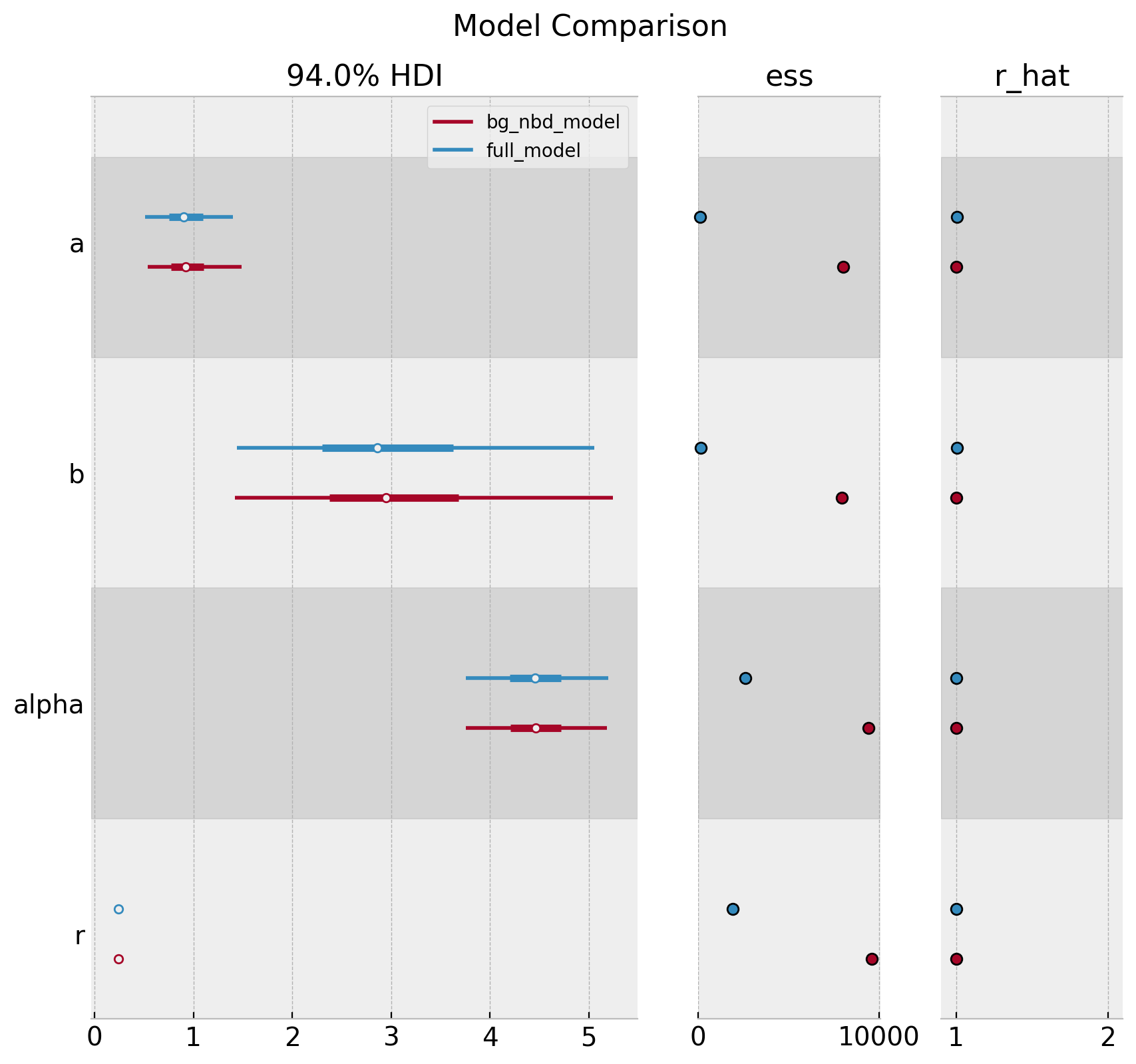
We indeed see that the full_model has a lower ess.
Bayesian Model: Randomly Chosen Individual with Time-Independent Covariates
In the research note Incorporating Time-Invariant Covariates into the Pareto/NBD and BG/NBD Models by Peter S. Fader and Bruce G. S. Hardie, it is shown how easy (after some clever math manipulations of course!) to incorporate time-invariant covariates into the BG/NBD model. The main idea is to allow covariates \(z_1\) and \(z_2\) to explain the cross-sectional heterogeneity in the purchasing process and cross-sectional heterogeneity in the dropout process respectively (see model description above). The authors show that the likelihood and quantities of interests computed by computing expectations (e.g. quantities which have a close expression so that, for example can be computed in Excel), remain almost the same. One only has to replace:
\[\begin{align*} \alpha & \longmapsto \alpha_{0}\exp(-\gamma_{1}^{T}z_{1}) \\ a & \longmapsto a_{0}\exp(\gamma_{2}^{T}z_{2}) \\ b & \longmapsto b_{0}\exp(\gamma_{3}^{T}z_{2}) \end{align*}\]
where \(\gamma_{i}\) are the model coefficients.
Let us modify the frequency of our data set by reducing it as a function of a covariate \(z\).
np.random.seed(42)

# construct covariate
mu = 0.4
rho = 0.7
z = rng.binomial(n=1, p=mu, size=x.size)
# change frequency values by reducing it the values where z !=0
x_z = np.floor(x * (1 - (rho * z)))
# make sure the recency is zero whenever the frequency is zero
t_x_z = t_x.copy()
t_x_z[np.argwhere(x_z == 0).flatten()] = 0
# sanity checks
assert x_z.min() == 0
assert np.all(t_x_z[np.argwhere(x_z == 0).flatten()] == 0)
# convenient indicator function
int_vec = np.vectorize(int)
x_zero_z = int_vec(x_z > 0)
First, we fit the lifetimes model with this modified data.
bgf_cov = BetaGeoFitter()
bgf_cov.fit(frequency=x_z, recency=t_x_z, T=T)

bgf_cov.summary| coef | se(coef) | lower 95% bound | upper 95% bound | |
|---|---|---|---|---|
| r | 0.142129 | 0.008739 | 0.125000 | 0.159258 |
| alpha | 4.252136 | 0.447587 | 3.374866 | 5.129407 |
| a | 0.750734 | 0.283204 | 0.195654 | 1.305815 |
| b | 3.157024 | 1.505522 | 0.206201 | 6.107846 |
Next, we write the bayesian model, which adds term \(\alpha \longmapsto \alpha_{0}\exp(-\gamma_{1}^{T}z_{1})\) to model the effect of \(z\) on the to explain the cross-sectional heterogeneity in the purchasing process (because we are modifying the frequency as a function of \(z\)).
Remark: I also tried adding the covariate \(z_2 = z\), but the resulting model had trouble sampling. By looking into the pair-plots of the posterior distributions (which had many divergences) I found that the terms \(a_0\) and \(b_0\) where highly correlated (actually, \(g_2\) (\(=\gamma_{2}\))and \(g_3\) (\(=\gamma_{3}\)) as well, see notation below). This indicates that we might need a different and more appropriate parametrization of the log-likelihood function.
with pm.Model() as model_cov:
    # a0 = pm.HalfNormal(name="a0", sigma=10)
    # g2 = pm.Normal(name="g2", mu=0, sigma=10)
    # a = a0 * tt.exp(g2 * z)
    a = pm.HalfNormal(name="a", sigma=10)

    # b0 = pm.HalfNormal(name="b0", sigma=10)
    # g3 = pm.Normal(name="g3", mu=0, sigma=10)
    # b = tt.exp(g3 * z)
    b = pm.HalfNormal(name="b", sigma=10)

    alpha0 = pm.HalfNormal(name="alpha0", sigma=10)
    g1 = pm.Normal(name="g1", mu=0, sigma=10)
    alpha = pm.Deterministic(name="alpha", var=alpha0 * pt.exp(-g1 * z))

    r = pm.HalfNormal(name="r", sigma=10)

    def logp(x, t_x, T, x_zero):
        a1 = pt.gammaln(r + x) - pt.gammaln(r) + r * pt.log(alpha)
        a2 = (
            pt.gammaln(a + b)
            + pt.gammaln(b + x)
            - pt.gammaln(b)
            - pt.gammaln(a + b + x)
        )
        a3 = -(r + x) * pt.log(alpha + T)
        a4 = (
            pt.log(a) - pt.log(b + pt.maximum(x, 1) - 1) - (r + x) * pt.log(t_x + alpha)
        )
        max_a3_a4 = pt.maximum(a3, a4)
        ll_1 = a1 + a2
        ll_2 = (
            pt.log(
                pt.exp(a3 - max_a3_a4)
                + pt.exp(a4 - max_a3_a4) * pm.math.switch(x_zero, 1, 0)
            )
            + max_a3_a4
        )
        return pt.sum(ll_1 + ll_2)

    likelihood = pm.Potential(
        name="likelihood",
        var=logp(x=x_z, t_x=t_x_z, T=T, x_zero=x_zero_z),
    )

pm.model_to_graphviz(model=model_cov)
with model_cov:
    trace_cov = pm.sample(
        tune=2_000,
        draws=4_000,
        chains=4,
        target_accept=0.95,
        nuts_sampler="numpyro",
    )
az.summary(data=trace_cov, var_names=["~alpha"])| mean | sd | hdi_3% | hdi_97% | mcse_mean | mcse_sd | ess_bulk | ess_tail | r_hat | |
|---|---|---|---|---|---|---|---|---|---|
| g1 | -2.860 | 0.141 | -3.133 | -2.606 | 0.001 | 0.001 | 15215.0 | 14112.0 | 1.0 |
| a | 1.175 | 0.571 | 0.380 | 2.192 | 0.006 | 0.004 | 10343.0 | 10398.0 | 1.0 |
| b | 5.264 | 3.162 | 1.321 | 10.998 | 0.033 | 0.024 | 10325.0 | 10249.0 | 1.0 |
| alpha0 | 4.024 | 0.434 | 3.232 | 4.854 | 0.004 | 0.003 | 11666.0 | 13128.0 | 1.0 |
| r | 0.226 | 0.015 | 0.198 | 0.253 | 0.000 | 0.000 | 12265.0 | 13506.0 | 1.0 |
axes = az.plot_trace(
    data=trace_cov,
    var_names=["~alpha"],
    lines=[(k, {}, [v]) for k, v in bgf_cov.summary["coef"].items()],
    compact=True,
    backend_kwargs={"figsize": (12, 15), "layout": "constrained"},
)
fig = axes[0][0].get_figure()
fig.suptitle(
    "BG/NBD Model (Time-Invariant Covariates) Trace", fontsize=16, fontweight="bold"
);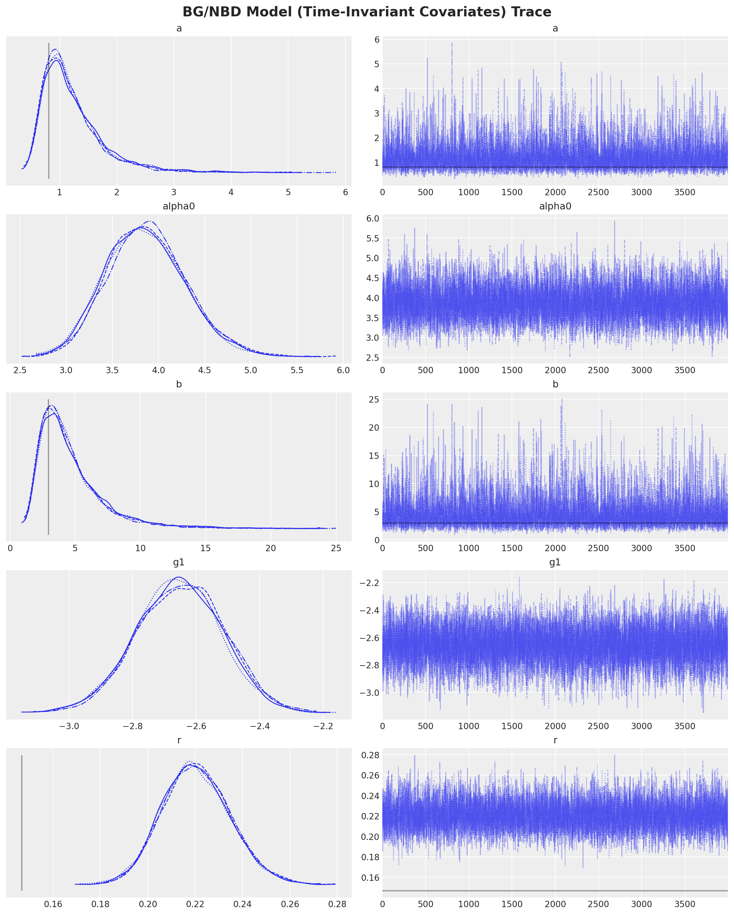
We indeed see a difference in the model parameters as compared with the model without covariates bgf_cov (note specially the shift in \(r\)).
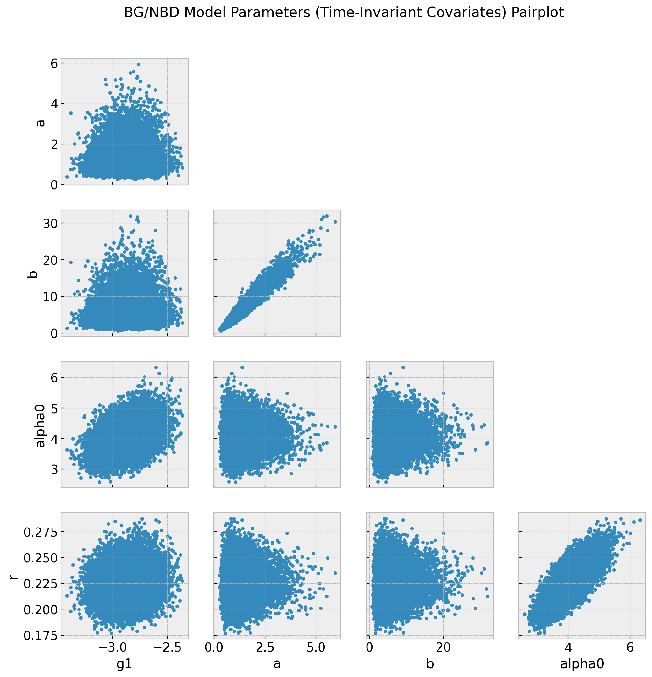
axes = az.plot_pair(data=trace_cov, var_names=["~alpha"], figsize=(12, 12))
fig = axes[0][0].get_figure()
fig.suptitle(
    "BG/NBD Model Parameters (Time-Invariant Covariates) Pairplot",
    fontsize=16,
    fontweight="bold",
);
Finally, let us see the two different values (for \(z=0\) and \(z=1\)) of the alpha parameter.
fig, ax = plt.subplots()
az.plot_dist(
    values=trace_cov.posterior["alpha"][:, :, z == 0].to_numpy().flatten(),
    color="C0",
    label=r"z = 0",
    ax=ax,
)
az.plot_dist(
    values=trace_cov.posterior["alpha"][:, :, z == 1].to_numpy().flatten(),
    color="C1",
    label=r"z = 1",
    ax=ax,
)
ax.legend(loc="upper right")
ax.set(title=r"$\alpha$ posterior", xlabel=r"$\alpha$", ylabel="count");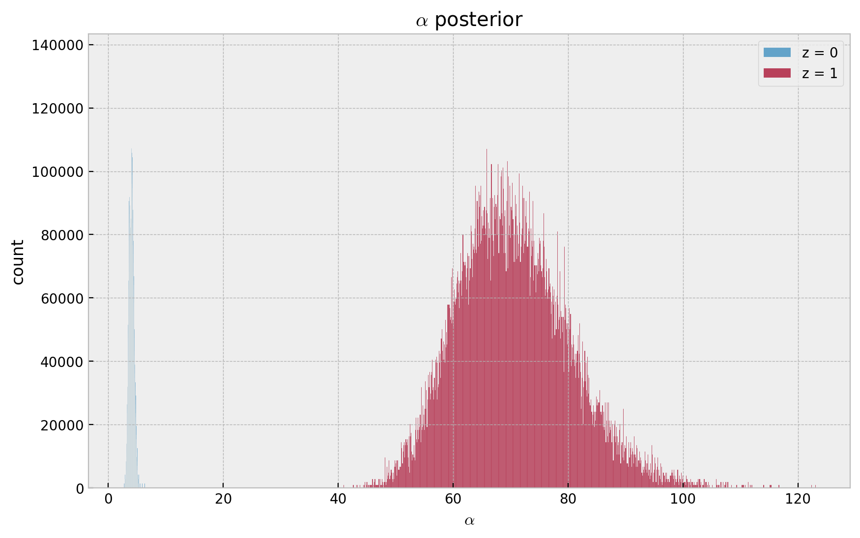
- Recall \(\lambda \sim \text{Gamma}(r, \alpha)\), which has expected value \(r/\alpha\).
- Hence, as \(g_1 < 0\), then \(\alpha(z=1) > \alpha(z=0)\) which is consistent with the data generation process where \(z = 1\) implied a lower frequency.
Bayesian Model: Hierarchical Model
In this final section we outline how to set up a hierarchical model. This is relevant when you want to model each user cohort separately. For example, you might want to model the purchasing behavior of users who joined the platform in April, May, June, etc. separately. This is useful because the purchasing behavior of users who joined the platform in April might be different from the purchasing behavior of users who joined the platform in June. However, they are not independent of each other hence we would like to pool information across cohorts. Moreover, this comes very handy when trying to make predictions for very young cohorts (cold start problem).
In this example we artificially create \(4\) cohorts:
groups = ["g1", "g2", "g3", "g4"]

data_df["group"] = rng.choice(a=groups, p=[0.45, 0.35, 0.15, 0.05], size=n_obs)

data_df["group"].value_counts()
g1 1065 g2 815 g3 353 g4 124 Name: group, dtype: int64
For the sake of comparison, let’s fit the lifetimes model each cohort.
group_summaries = []

for g, group_df in data_df.groupby("group"):
    # set data
    x_g = group_df["frequency"].to_numpy()
    t_x_g = group_df["recency"].to_numpy()
    T_g = group_df["T"].to_numpy()
    x_zero_g = int_vec(x_g > 0)
    # fit model
    bgf_g = BetaGeoFitter()
    bgf_g.fit(frequency=x_g, recency=t_x_g, T=T_g)
    group_summary_df = (
        bgf_g.summary.assign(group=g)
        .reset_index(drop=False)
        .rename(columns={"index": "parameter"})
    )
    group_summaries.append(group_summary_df)

group_summaries = pd.concat(group_summaries, axis=0).reset_index(drop=True)group_summaries| parameter | coef | se(coef) | lower 95% bound | upper 95% bound | group | |
|---|---|---|---|---|---|---|
| 0 | r | 0.230703 | 0.017721 | 0.195971 | 0.265436 | g1 |
| 1 | alpha | 4.312733 | 0.547934 | 3.238784 | 5.386683 | g1 |
| 2 | a | 0.989651 | 0.415796 | 0.174691 | 1.804611 | g1 |
| 3 | b | 3.291437 | 1.724476 | -0.088537 | 6.671411 | g1 |
| 0 | r | 0.259025 | 0.022853 | 0.214233 | 0.303816 | g2 |
| 1 | alpha | 4.754671 | 0.684570 | 3.412914 | 6.096428 | g2 |
| 2 | a | 0.564523 | 0.185246 | 0.201440 | 0.927606 | g2 |
| 3 | b | 1.457592 | 0.586177 | 0.308686 | 2.606499 | g2 |
| 0 | r | 0.271790 | 0.037150 | 0.198976 | 0.344603 | g3 |
| 1 | alpha | 4.781757 | 1.090382 | 2.644607 | 6.918906 | g3 |
| 2 | a | 2.327516 | 3.830876 | -5.181000 | 9.836032 | g3 |
| 3 | b | 10.054263 | 18.778442 | -26.751482 | 46.860009 | g3 |
| 0 | r | 0.180750 | 0.039690 | 0.102958 | 0.258542 | g4 |
| 1 | alpha | 2.806377 | 1.095709 | 0.658788 | 4.953967 | g4 |
| 2 | a | 0.821841 | 0.646647 | -0.445587 | 2.089269 | g4 |
| 3 | b | 2.217292 | 2.128679 | -1.954919 | 6.389502 | g4 |
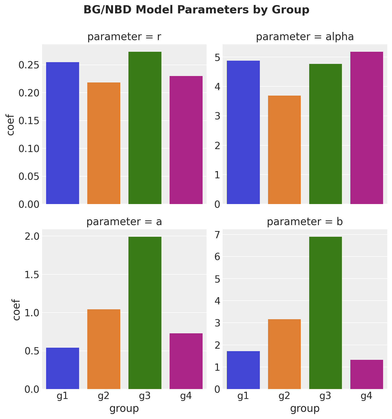
g = sns.catplot(
    data=group_summaries,
    x="group",
    y="coef",
    hue="group",
    col="parameter",
    col_wrap=2,
    kind="bar",
    sharex=True,
    sharey=False,
    height=4,
)

g.figure.suptitle(
    "BG/NBD Model Parameters by Group", y=1.05, fontsize=16, fontweight="bold"
);
Now we specify the hierarchical model.
group_idx, groups = data_df["group"].factorize(sort=True)

coords = {
    "group_idx": group_idx,
    "group": groups,
}

with pm.Model(coords=coords) as model_h:
    # hyper-priors
    alpha_a = pm.Gamma(name="alpha_a", alpha=1, beta=1)
    beta_a = pm.Gamma(name="beta_a", alpha=1, beta=1)
    alpha_b = pm.Gamma(name="alpha_b", alpha=1, beta=1)
    beta_b = pm.Gamma(name="beta_b", alpha=1, beta=1)

    alpha_alpha = pm.Gamma(name="alpha_alpha", alpha=5, beta=2)
    beta_alpha = pm.Gamma(name="beta_alpha", alpha=2, beta=2)
    alpha_r = pm.Gamma(name="alpha_r", alpha=1, beta=1)
    beta_r = pm.Gamma(name="beta_r", alpha=1, beta=1)

    # priors
    a_group = pm.Gamma(name="a", alpha=alpha_a, beta=beta_a, dims="group")
    b_group = pm.Gamma(name="b", alpha=alpha_b, beta=beta_b, dims="group")

    alpha_group = pm.Gamma(
        name="alpha", alpha=alpha_alpha, beta=beta_alpha, dims="group"
    )
    r_group = pm.Gamma(name="r", alpha=alpha_r, beta=beta_r, dims="group")

    # cohort-specific parameters
    a = a_group[group_idx]
    b = b_group[group_idx]
    alpha = alpha_group[group_idx]
    r = r_group[group_idx]

    # log-likelihood
    def logp(x, t_x, T, x_zero):
        a1 = pt.gammaln(r + x) - pt.gammaln(r) + r * pt.log(alpha)
        a2 = (
            pt.gammaln(a + b)
            + pt.gammaln(b + x)
            - pt.gammaln(b)
            - pt.gammaln(a + b + x)
        )
        a3 = -(r + x) * pt.log(alpha + T)
        a4 = (
            pt.log(a) - pt.log(b + pt.maximum(x, 1) - 1) - (r + x) * pt.log(t_x + alpha)
        )
        max_a3_a4 = pt.maximum(a3, a4)
        ll_1 = a1 + a2
        ll_2 = (
            pt.log(
                pt.exp(a3 - max_a3_a4)
                + pt.exp(a4 - max_a3_a4) * pm.math.switch(x_zero, 1, 0)
            )
            + max_a3_a4
        )
        return pt.sum(ll_1 + ll_2)

    likelihood = pm.Potential(name="likelihood", var=logp(x, t_x, T, x_zero))


pm.model_to_graphviz(model=model_h)
with model_h:
    trace_h = pm.sample(
        tune=2_000,
        draws=4_000,
        chains=4,
        target_accept=0.95,
        nuts_sampler="numpyro",
    )
axes = az.plot_trace(
data=trace_h,
var_names=["a", "b", "alpha", "r"],
lines=[(k, {}, [v]) for k, v in bgf.summary["coef"].items()],
compact=True,
backend_kwargs={
"figsize": (12, 9),
"layout": "constrained"
},
)
fig = axes[0][0].get_figure()
fig.suptitle("Hierarchical BG/NBD Model Trace", fontsize=16);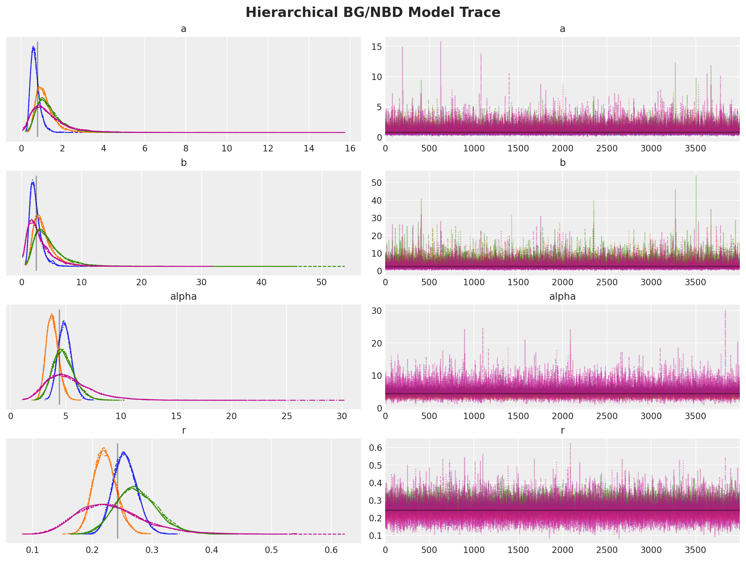
Let’s look into the summary:
az.summary(data=trace_h)| mean | sd | hdi_3% | hdi_97% | mcse_mean | mcse_sd | ess_bulk | ess_tail | r_hat | |
|---|---|---|---|---|---|---|---|---|---|
| alpha_a | 1.686 | 0.869 | 0.345 | 3.308 | 0.006 | 0.004 | 19833.0 | 15505.0 | 1.0 |
| beta_a | 1.610 | 0.964 | 0.113 | 3.346 | 0.007 | 0.005 | 18769.0 | 13989.0 | 1.0 |
| alpha_b | 2.158 | 1.177 | 0.376 | 4.334 | 0.008 | 0.006 | 19374.0 | 14736.0 | 1.0 |
| beta_b | 0.727 | 0.492 | 0.035 | 1.612 | 0.004 | 0.003 | 14664.0 | 14192.0 | 1.0 |
| alpha_alpha | 3.356 | 1.157 | 1.426 | 5.586 | 0.007 | 0.005 | 24029.0 | 16938.0 | 1.0 |
| beta_alpha | 0.806 | 0.326 | 0.253 | 1.424 | 0.002 | 0.001 | 23975.0 | 16880.0 | 1.0 |
| alpha_r | 0.985 | 0.490 | 0.203 | 1.884 | 0.003 | 0.002 | 24218.0 | 15896.0 | 1.0 |
| beta_r | 2.523 | 1.499 | 0.208 | 5.237 | 0.009 | 0.007 | 24994.0 | 15206.0 | 1.0 |
| a[g1] | 1.073 | 0.427 | 0.444 | 1.820 | 0.004 | 0.003 | 17394.0 | 13936.0 | 1.0 |
| a[g2] | 0.719 | 0.252 | 0.323 | 1.185 | 0.002 | 0.001 | 21337.0 | 16544.0 | 1.0 |
| a[g3] | 1.171 | 0.653 | 0.288 | 2.296 | 0.005 | 0.004 | 16840.0 | 15148.0 | 1.0 |
| a[g4] | 1.053 | 0.604 | 0.196 | 2.121 | 0.005 | 0.003 | 17540.0 | 17338.0 | 1.0 |
| b[g1] | 3.732 | 1.897 | 1.223 | 7.015 | 0.016 | 0.012 | 17363.0 | 13250.0 | 1.0 |
| b[g2] | 2.046 | 0.922 | 0.733 | 3.723 | 0.007 | 0.005 | 21084.0 | 16081.0 | 1.0 |
| b[g3] | 4.662 | 3.055 | 0.865 | 9.795 | 0.026 | 0.019 | 16142.0 | 14831.0 | 1.0 |
| b[g4] | 3.354 | 2.367 | 0.464 | 7.385 | 0.019 | 0.013 | 17720.0 | 16726.0 | 1.0 |
| alpha[g1] | 4.348 | 0.547 | 3.375 | 5.414 | 0.003 | 0.002 | 25730.0 | 19111.0 | 1.0 |
| alpha[g2] | 4.770 | 0.675 | 3.571 | 6.068 | 0.004 | 0.003 | 26851.0 | 19591.0 | 1.0 |
| alpha[g3] | 4.764 | 1.027 | 2.895 | 6.659 | 0.006 | 0.005 | 25637.0 | 18370.0 | 1.0 |
| alpha[g4] | 3.352 | 1.132 | 1.402 | 5.454 | 0.007 | 0.005 | 25535.0 | 19124.0 | 1.0 |
| r[g1] | 0.232 | 0.018 | 0.197 | 0.264 | 0.000 | 0.000 | 26531.0 | 19190.0 | 1.0 |
| r[g2] | 0.259 | 0.023 | 0.218 | 0.303 | 0.000 | 0.000 | 26711.0 | 20014.0 | 1.0 |
| r[g3] | 0.272 | 0.036 | 0.205 | 0.338 | 0.000 | 0.000 | 25764.0 | 18768.0 | 1.0 |
| r[g4] | 0.195 | 0.040 | 0.123 | 0.272 | 0.000 | 0.000 | 25393.0 | 19000.0 | 1.0 |
Finally, let’s compare the parameter of the lifetimes model with the predictions of the hierarchical model.
fig, axes = plt.subplots(
    nrows=2, ncols=2, figsize=(15, 15), sharex=False, sharey=False, layout="constrained"
)

axes = axes.flatten()

for i, parameter in enumerate(["r", "alpha", "a", "b"]):
    # compute summary per parameter
    parameter_hdi = az.hdi(trace_h.posterior[parameter])[parameter].to_numpy()
    parameter_mean = (
        trace_h.posterior[parameter].stack(sample=("chain", "draw")).mean(axis=1)
    )

    model_h_parameter_df = pd.DataFrame(
        data=parameter_hdi, columns=["lower", "upper"]
    ).assign(group=groups, mean=parameter_mean)

    lifetimes_parameter_df = group_summaries.query("parameter == @parameter")

    parameter_df = model_h_parameter_df.merge(lifetimes_parameter_df, on="group")

    # plot
    ax = axes[i]

    for j, row in parameter_df.iterrows():

        ax.vlines(
            x=row["coef"],
            ymin=row["lower 95% bound"],
            ymax=row["upper 95% bound"],
            color=f"C{j}",
            label=row["group"],
            alpha=0.7,
        )
        ax.hlines(
            y=row["mean"],
            xmin=row["lower"],
            xmax=row["upper"],
            color=f"C{j}",
            alpha=0.7,
        )

        ax.scatter(x=row["coef"], y=row["mean"], color=f"C{j}", s=80)

    ax.axline(
        xy1=(row["mean"], row["mean"]),
        slope=1,
        color="black",
        linestyle="--",
        label="diagonal",
    )
    ax.axvline(
        x=bgf.summary.reset_index(drop=False)
        .query("index == @parameter")["coef"]
        .item(),
        color="gray",
        linestyle="--",
        label="lifetimes (global)",
    )
    ax.axhline(
        y=bgf.summary.reset_index(drop=False)
        .query("index == @parameter")["coef"]
        .item(),
        color="gray",
        linestyle="--",
    )
    ax.legend(loc="lower right")

    ax.set(title=parameter, xlabel="lifetimes", ylabel="hierarchical model")

fig.suptitle(
    "Parameters - Hierarchical BG/NBD Model vs. Lifetimes",
    fontsize=20,
    fontweight="bold",
);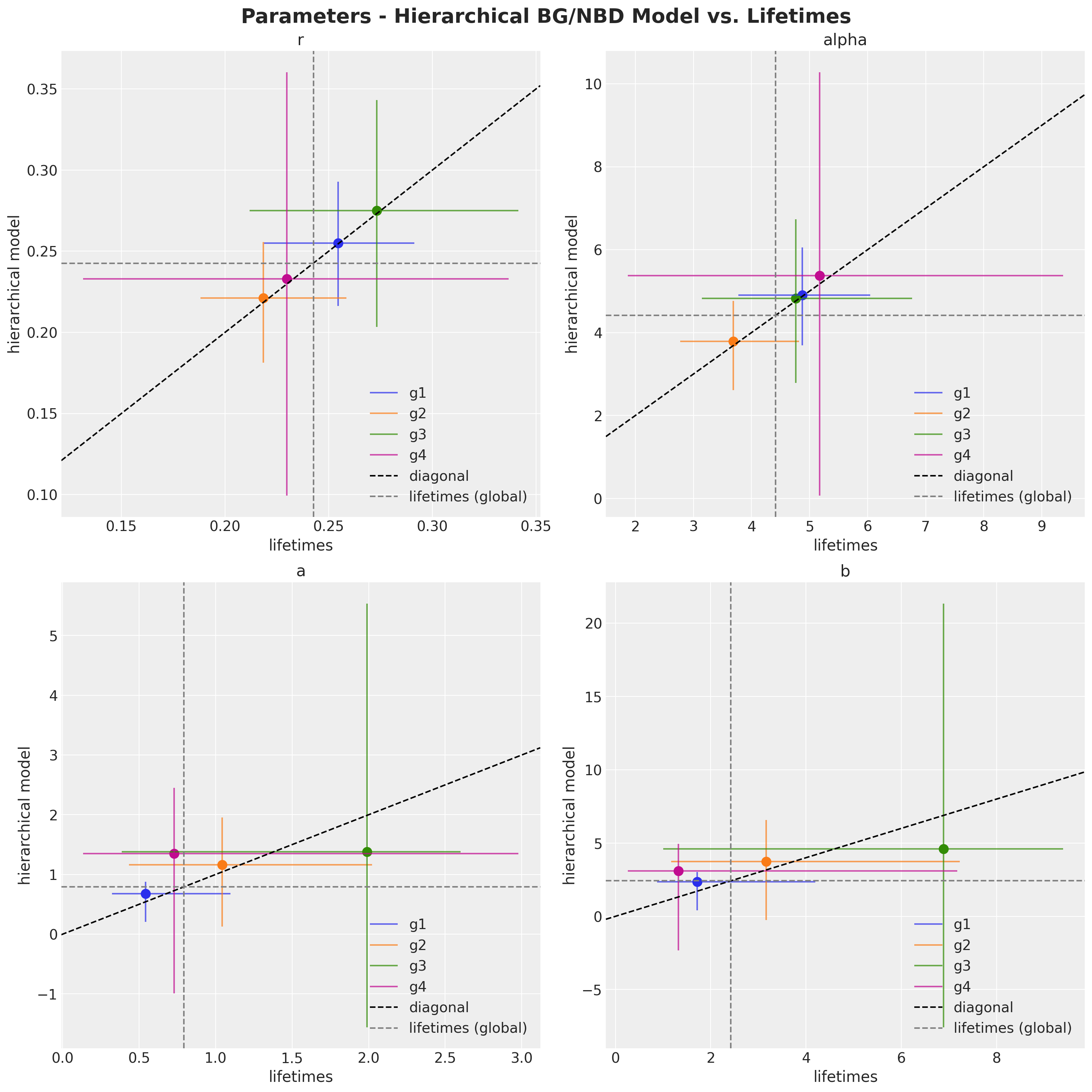
Here we can see the shrinkage effect of the hierarchical model. The model parameters are closer to the global estimates (i.e. the estimates of the model without cohorts).