Introduction to BTYD (Buy Until You Die) Models

Berlin Bayesians MeetUp - September 2022

Dr. Juan Orduz

Outline

1. Introduction to BTYD Models

2. BG/NBD Model: Model Specification

3. BG/NBD Model: Maximum Likelihood Estimation (lifetimes)

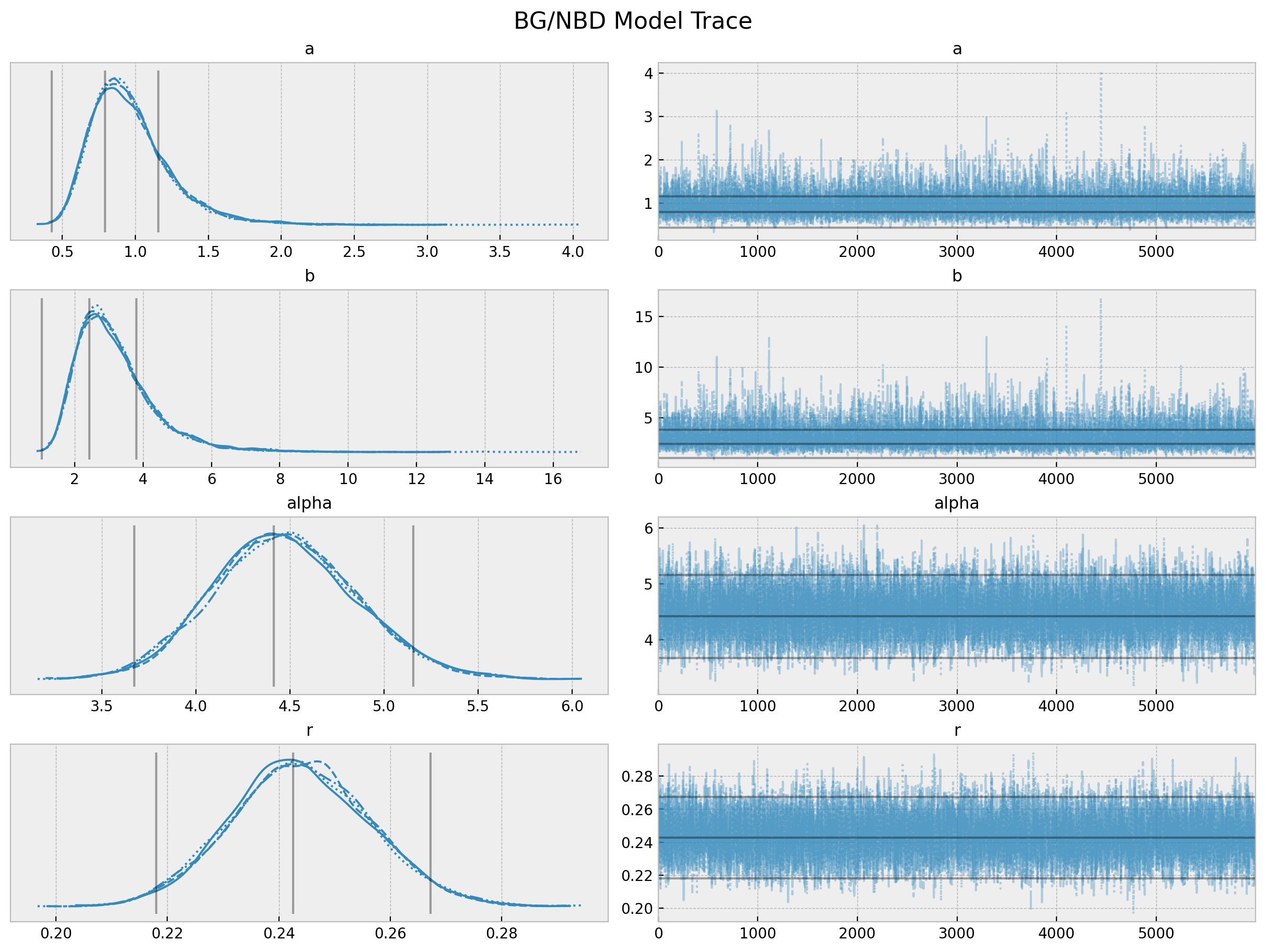
4. BG/NBD Model: Bayesian Estimation (pymc)

   • External Regressors
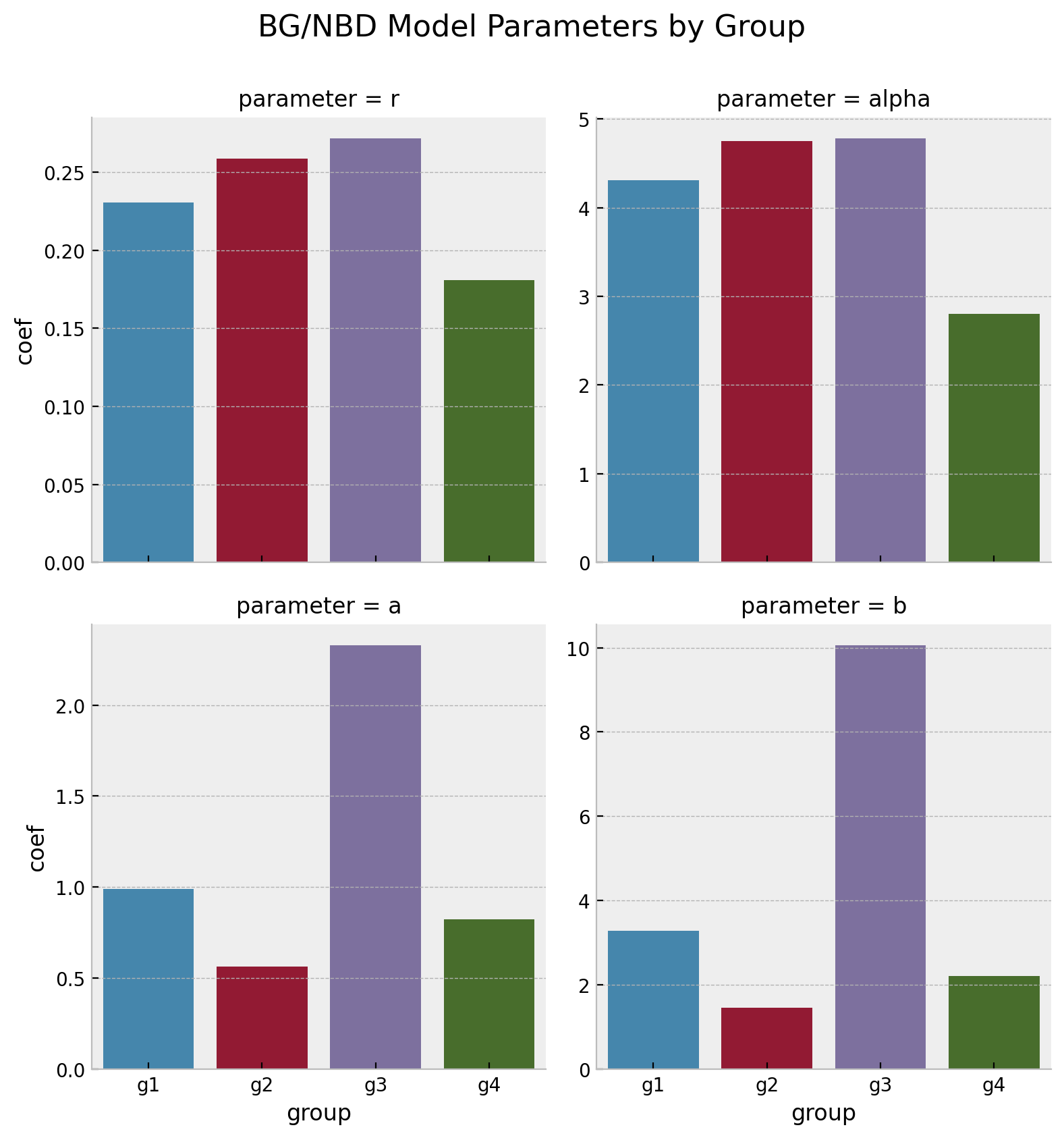
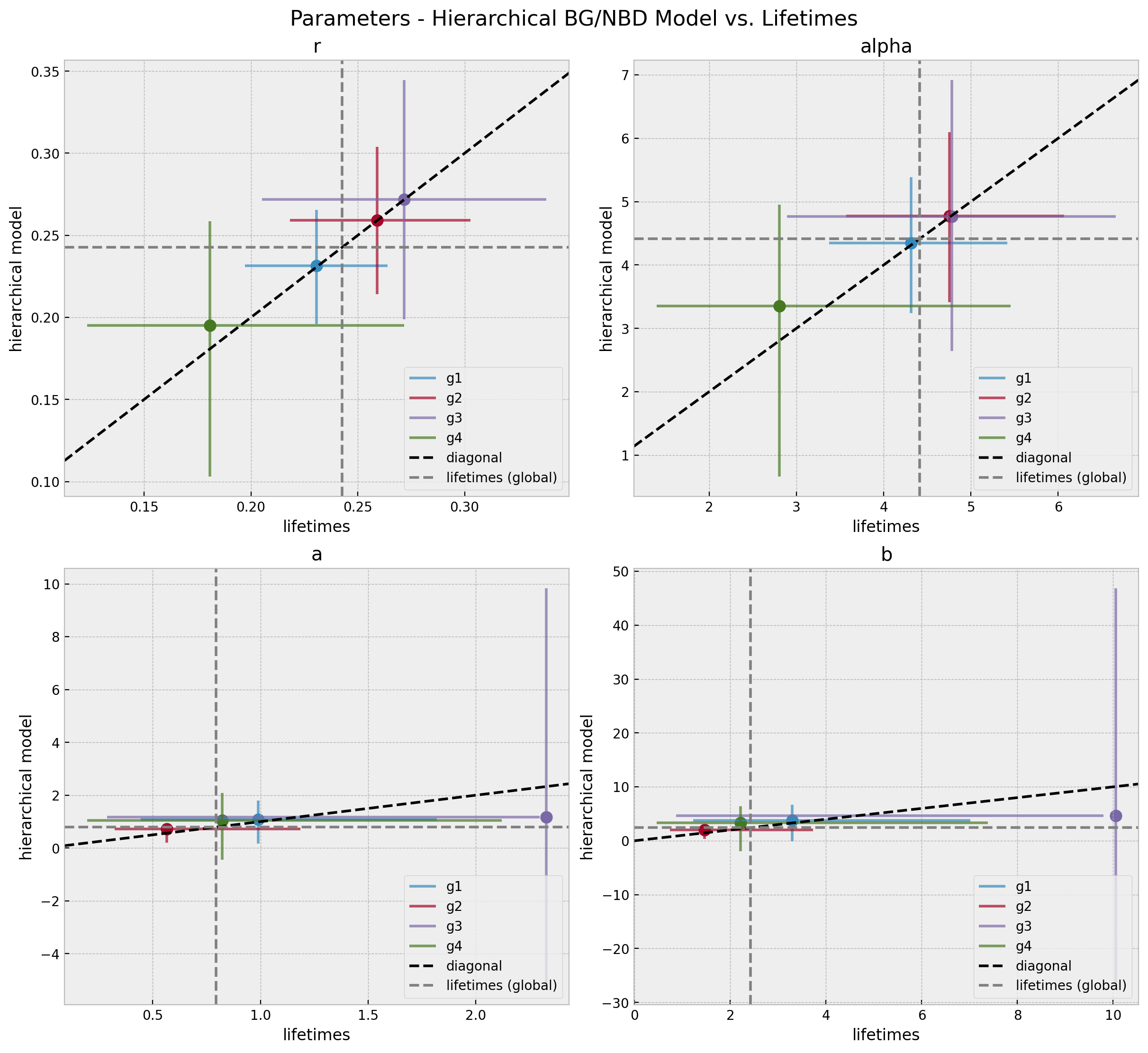
   • Hierarchical Model

5. References and Resources

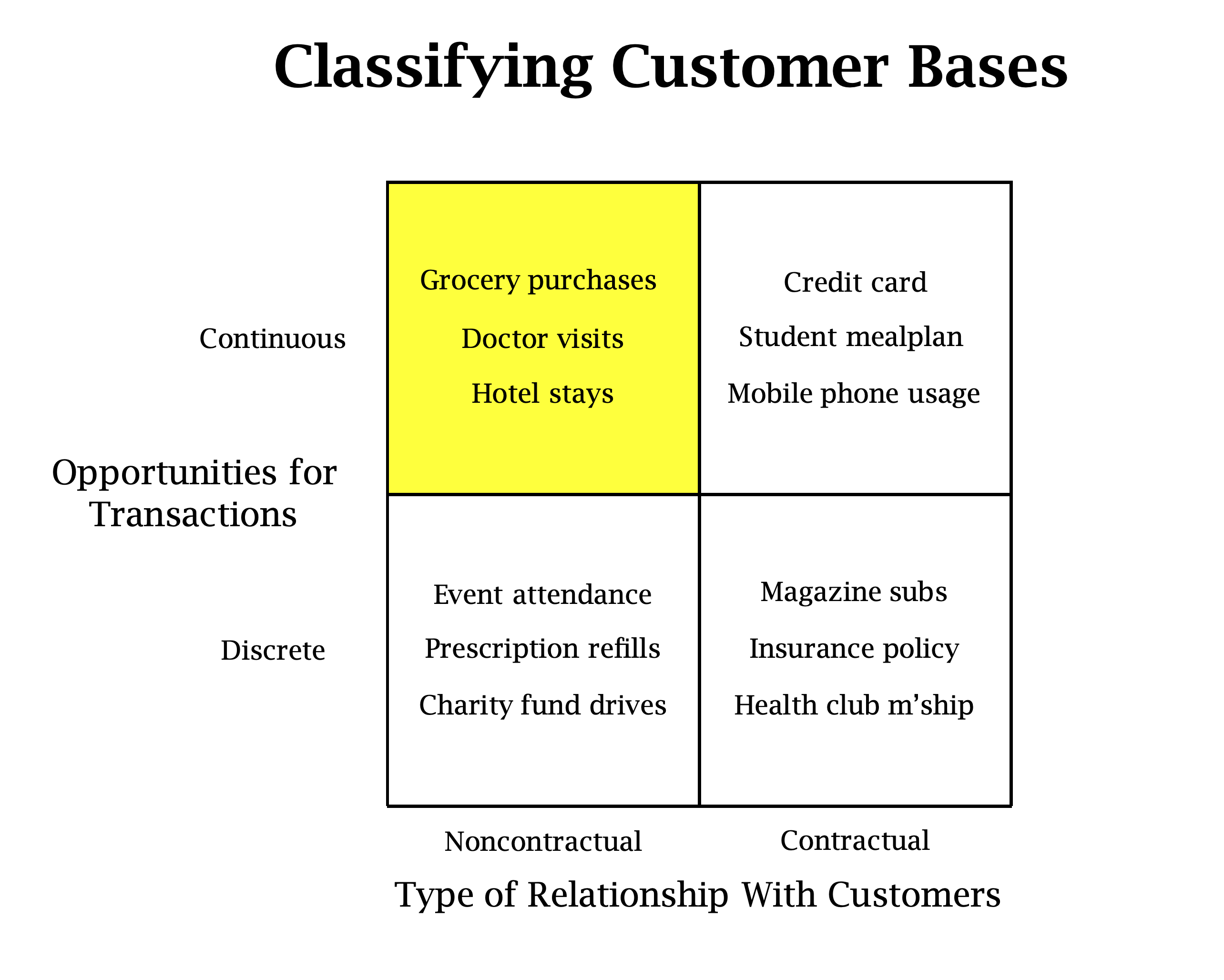
Classifying Customer Bases

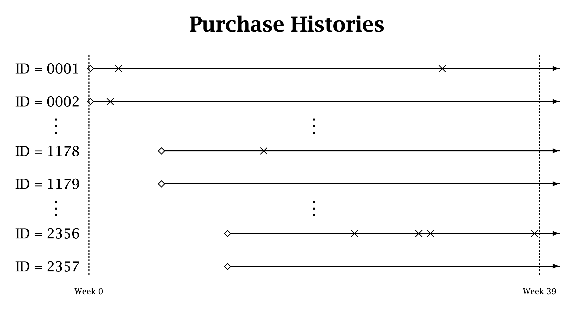
Purchase Histories

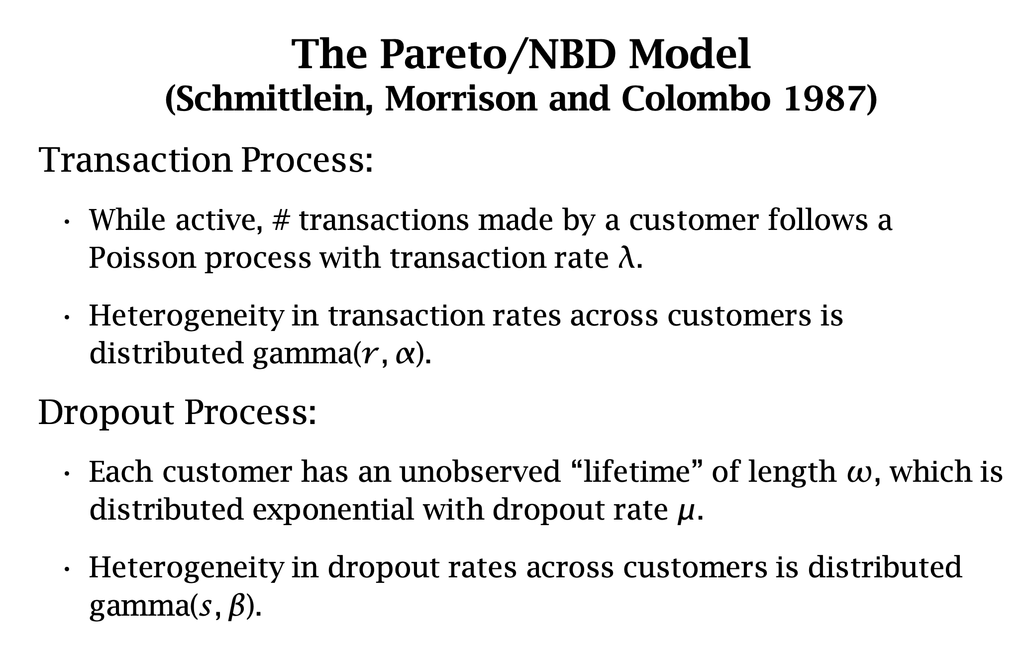
The Pareto/NBD Model

Models Workflow

%%{init: {"theme": "dark", "themeVariables": {"fontSize": "12px"}, "flowchart":{"htmlLabels":false}}}%%


flowchart LR
  A["Transaction Data"] --> B("Transaction Model - BG/NBD")
  A --> C("Monetary Model - GG")
  B --> D["Probability of Alive"]
  B --> E["Predicted Frequency"]
  C --> F["Predicted Avg. Monetary Value"]
  E --> G["Predicted CLV"]
  F --> G

• Transaction Model: Number of transactions per customer.
• Monetary Model: Average monetary value of a transaction.

CLV Formula

Discounted cash flow (DCF) method:

\[ CLV = \sum_{i=1}^{\infty} \frac{M_i}{(1+\delta)^i} \]

• \(M_{i}\): cash flow in period \(i\).
• \(\delta\): discount rate.

for i in steps:
    df["clv"] += (
        (monetary_value * expected_number_of_transactions) 
        / (1 + discount_rate) ** i 
    )

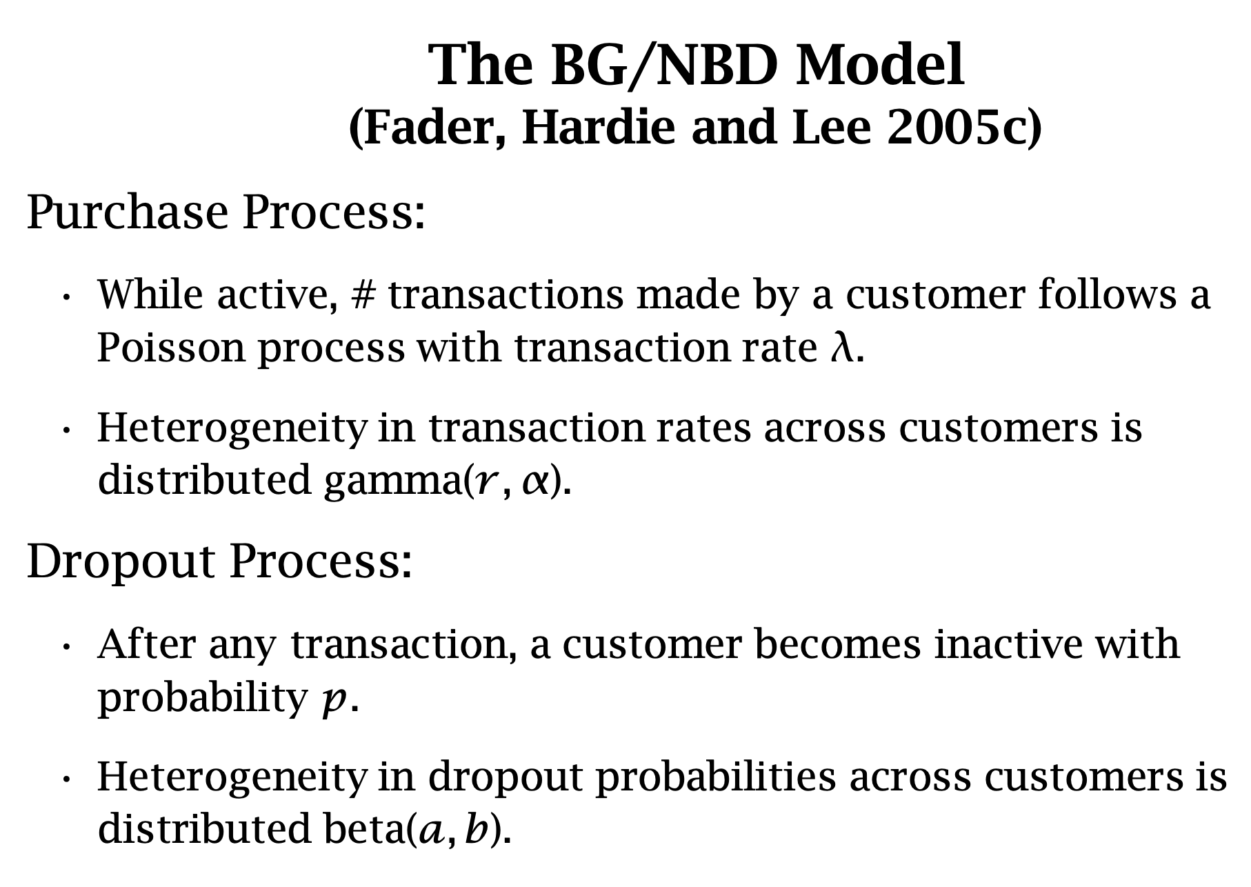
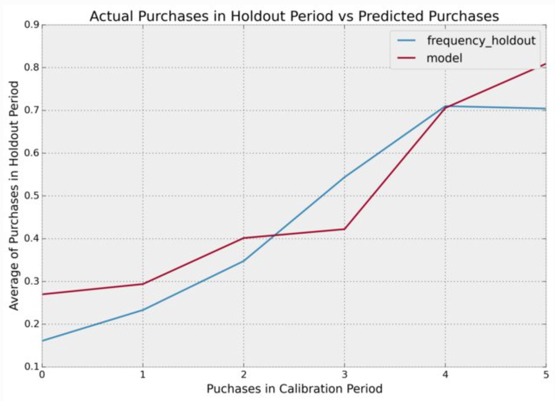
The BG/NBD Transaction Model

Purchase Metrics

• frequency: Number of repeat purchases the customer has made. More precisely, It’s the count of time periods the customer had a purchase in.

• T: Age of the customer in whatever time units chosen. This is equal to the duration between a customer’s first purchase and the end of the period under study.

• recency: Age of the customer when they made their most recent purchases. This is equal to the duration between a customer’s first purchase and their latest purchase.

BG/NBD Assumptions (Frequency)

1. While active, the time between transactions is distributed exponential with transaction rate, i.e.,

   \[f(t_{j}|t_{j-1}; \lambda) = \lambda \exp(-\lambda (t_{j} - t_{j - 1})), \quad t_{j} \geq t_{j - 1} \geq 0\]

2. Heterogeneity in \(\lambda\) follows a gamma distribution with pdf

   \[f(\lambda|r, \alpha) = \frac{\alpha^{r}\lambda^{r - 1}\exp(-\lambda \alpha)}{\Gamma(r)}, \quad \lambda > 0\]

BG/NBD Assumptions (Dropout)

3. After any transaction, a customer becomes inactive with probability \(p\).

4. Heterogeneity in \(p\) follows a beta distribution with pdf

   \[f(p|a, b) = \frac{\Gamma(a + b)}{\Gamma(a) \Gamma(b)} p^{a - 1}(1 - p)^{b - 1}, \quad 0 \leq p \leq 1\]

5. The transaction rate \(\lambda\) and the dropout probability \(p\) vary independently across customers.

Likelihood: Easy to Compute!

\[ L(a, b, \alpha, r|X=x, t_x, T) = A_{1}A_{2}(A_{3} + \delta_{x>0}A_4) \]

where

\[\begin{align*} A_{1} = \frac{\Gamma(r + x)\alpha^{{r}}}{\Gamma(x)} \quad A_{2} & = \frac{\Gamma(a + b)\Gamma(b + x)}{\Gamma(b)\Gamma(a + b + x)} \\ A_{3} = \left(\frac{1}{\alpha + T}\right)^{r+x} \quad A_{4} & = \left(\frac{a}{b + x - 1}\right)\left(\frac{1}{\alpha + t_x}\right)^{r + x} \end{align*}\]

Strategy: Write this in numpy as pass it through scipy.optimize.minimize

Inference: lifetimes Package

The four BG/NBD model parameters can be estimated via the method of maximum likelihood.

import numpy as np
import pandas as pd
from lifetimes.datasets import load_cdnow_summary
from lifetimes import BetaGeoFitter

data_df: pd.DataFrame = load_cdnow_summary(index_col=[0])

n = data_df.shape[0]
x = data_df["frequency"].to_numpy()
t_x = data_df["recency"].to_numpy()
T = data_df["T"].to_numpy()

bgf = BetaGeoFitter()
bgf.fit(frequency=x, recency=t_x, T=T)

Predicted Future Purchases

from lifetimes.plotting import plot_frequency_recency_matrix

ax = plot_frequency_recency_matrix(model=bgf, T=15)

\[E[Y(t) | X=x, t_x, T, r, \alpha, a , b]\]

Probability of Alive

from lifetimes.plotting import plot_probability_alive_matrix

ax = plot_probability_alive_matrix(model=bgf)

Probability of Alive

Model Evaluation

summary["model_predictions"] = model.conditional_expected_number_of_purchases_up_to_time(
    duration_holdout, summary["frequency_cal"], summary["recency_cal"], summary["T_cal"]
)

summary.groupby("frequency_cal")[["frequency_holdout", "model_predictions"]].mean().plot()

From Numpy to Aesara

We can re-write the numpy likelihood implementation in aesara.

Log-Likelihood in Aesara

The translation bewtween numpy and aesara is very easy (replace np by at)!

import aesara.tensor as at


def logp(x, t_x, T, x_zero):
    a1 = at.gammaln(r + x) - at.gammaln(r) + r * at.log(alpha)
    a2 = (
        at.gammaln(a + b)
        + at.gammaln(b + x)
        - at.gammaln(b)
        - at.gammaln(a + b + x)
    )
    a3 = -(r + x) * at.log(alpha + T)
    a4 = (
        at.log(a) - at.log(b + at.maximum(x, 1) - 1) - (r + x) * at.log(t_x + alpha)
    )
    max_a3_a4 = at.maximum(a3, a4)
    ll_1 = a1 + a2
    ll_2 = (
        at.log(
            at.exp(a3 - max_a3_a4)
            + at.exp(a4 - max_a3_a4) * pm.math.switch(x_zero, 1, 0)
        )
        + max_a3_a4
    )
    return at.sum(ll_1 + ll_2)

BG/NBD PyMC Model

Model Structure

import pymc as pm
import pymc.sampling_jax


with pm.Model() as model:

    a = pm.HalfNormal(name="a", sigma=10)
    b = pm.HalfNormal(name="b", sigma=10)

    alpha = pm.HalfNormal(name="alpha", sigma=10)
    r = pm.HalfNormal(name="r", sigma=10)

    def logp(x, t_x, T, x_zero):
        ...

    likelihood = pm.Potential(
        name="likelihood",
        var=logp(x=x, t_x=t_x, T=T, x_zero=x_zero),
    )

Model Sampling

with model:
    trace = pm.sampling_jax.sample_numpyro_nuts(
        tune=3000, draws=6000, chains=4,target_accept=0.95
)

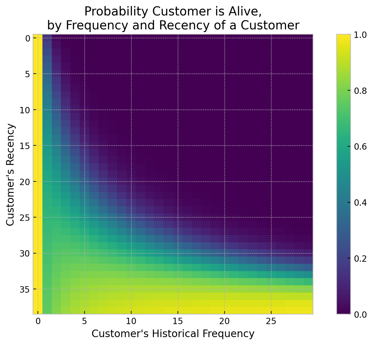
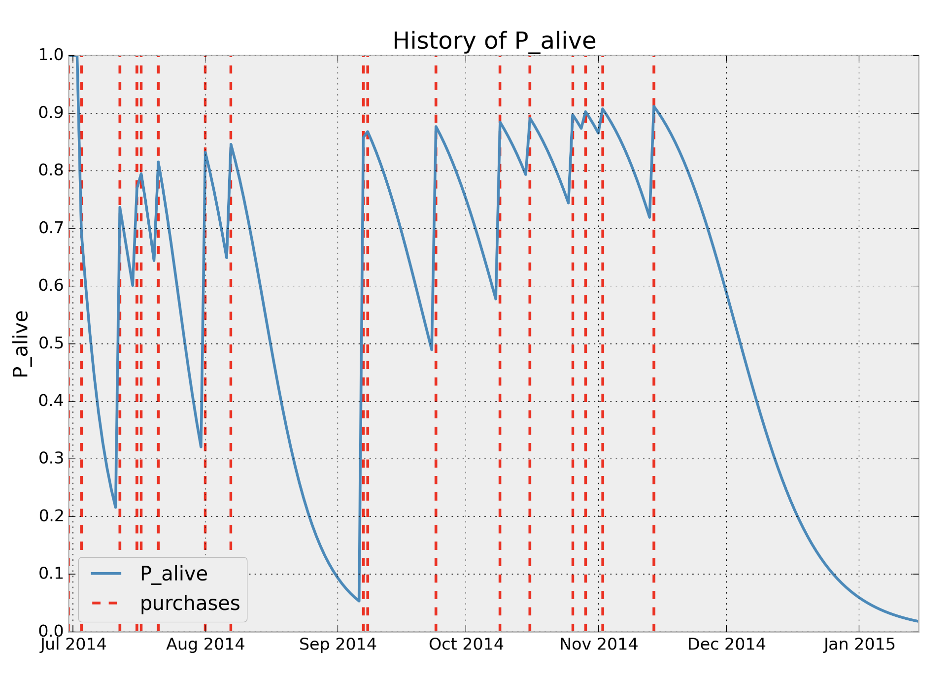
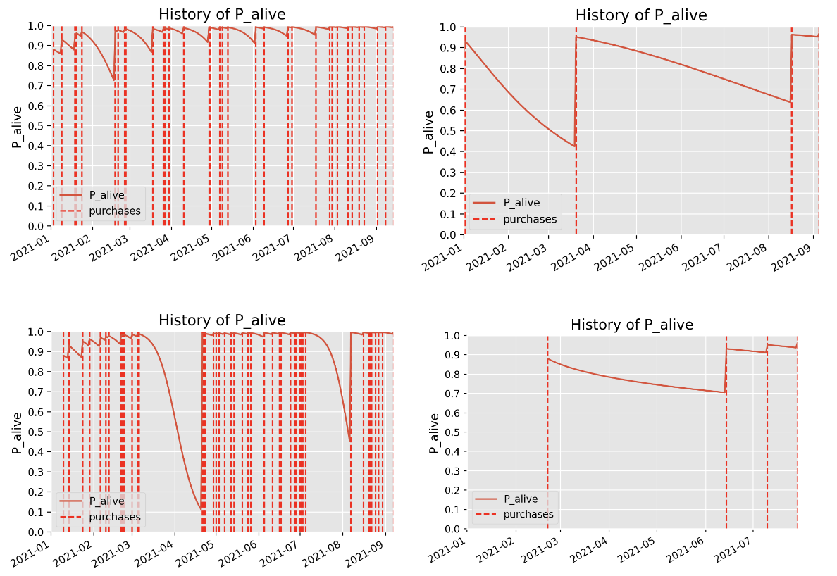
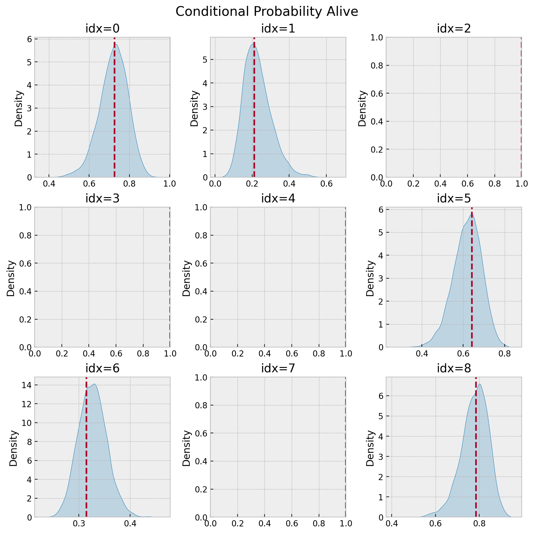
Probability of Active

How? Simply use the posterior samples (xarray) and broadcast the numpy expressions.

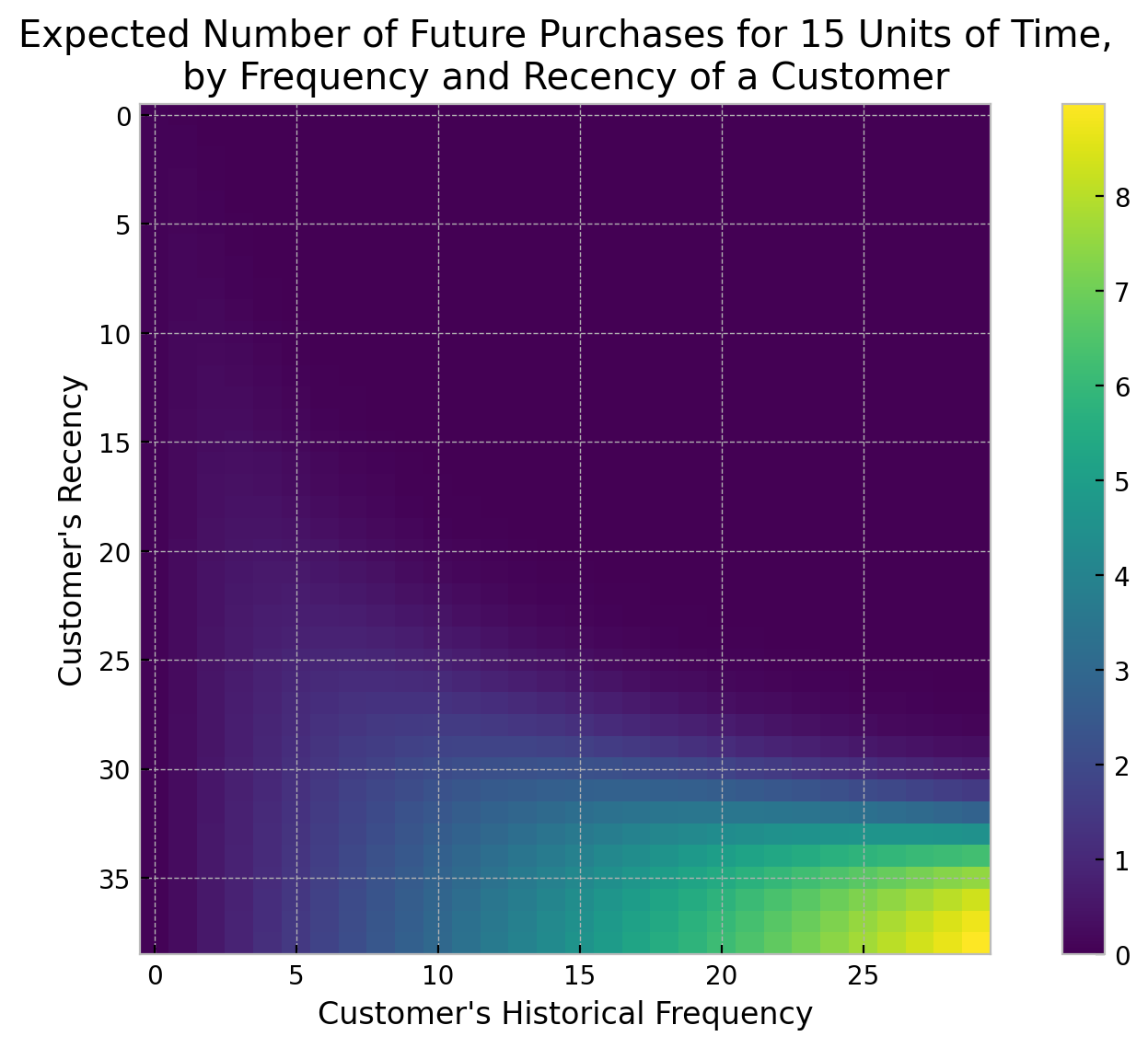
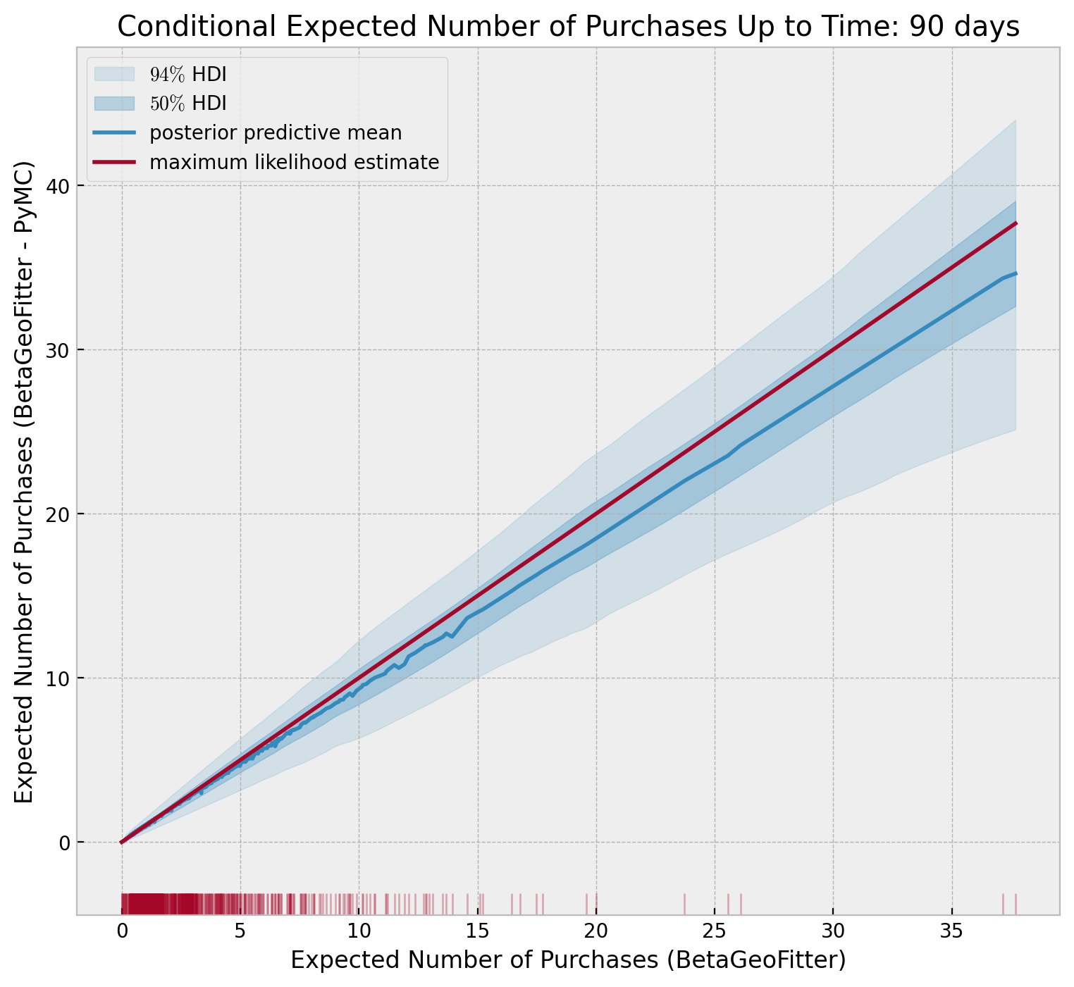
Future Purchases

Similarty, using the analytical expressions:

Time-Independent Covariates?

• Allow covariates \(z_1\) and \(z_2\) to explain the cross-sectional heterogeneity in the purchasing process and cross-sectional heterogeneity in the dropout process respectively.

• The likelihood and quantities of interests computed by computing expectations, remain almost the same. One only has to replace:

\[\begin{align*} \alpha & \longmapsto \alpha_{0}\exp(-\gamma_{1}^{T}z_{1}) \\ a & \longmapsto a_{0}\exp(\gamma_{2}^{T}z_{2}) \\ b & \longmapsto b_{0}\exp(\gamma_{3}^{T}z_{2}) \end{align*}\]

Simulated Example

np.random.seed(42)

# construct covariate
mu = 0.4
rho = 0.7
z = np.random.binomial(n=1, p=mu, size=x.size)

# change frequency values by reducing it the values where z !=0
x_z = np.floor(x * (1 - (rho * z)))

# make sure the recency is zero whenever the frequency is zero
t_x_z = t_x.copy()
t_x_z[np.argwhere(x_z == 0).flatten()] = 0

# sanity checks
assert x_z.min() == 0
assert np.all(t_x_z[np.argwhere(x_z == 0).flatten()] == 0)

\(z = 1 \Rightarrow\) the frequency is reduced by \(70\%\).

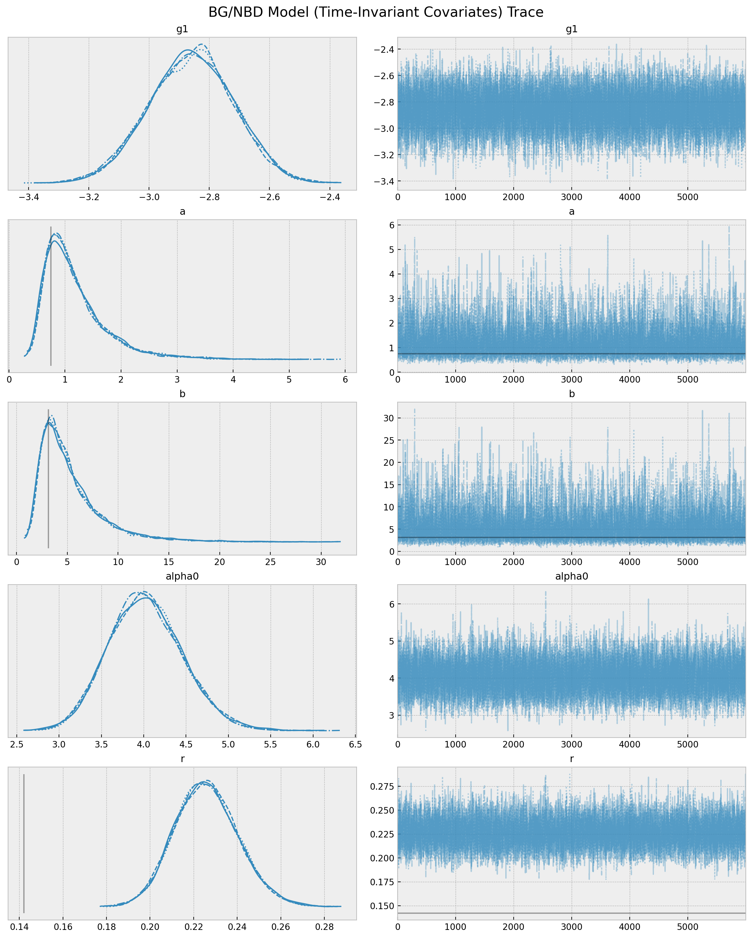
PyMC Model

with pm.Model() as model_cov:

    a = pm.HalfNormal(name="a", sigma=10)
    b = pm.HalfNormal(name="b", sigma=10)

    alpha0 = pm.HalfNormal(name="alpha0", sigma=10)
    g1 = pm.Normal(name="g1", mu=0, sigma=10)
    alpha = pm.Deterministic(name="alpha", var=alpha0 * at.exp(- g1 * z))
    
    r = pm.HalfNormal(name="r", sigma=10)

    def logp(x, t_x, T, x_zero):
        ...

    likelihood = pm.Potential(
        name="likelihood",
        var=logp(x=x_z, t_x=t_x_z, T=T, x_zero=x_zero_z),
    )

Model Parameters

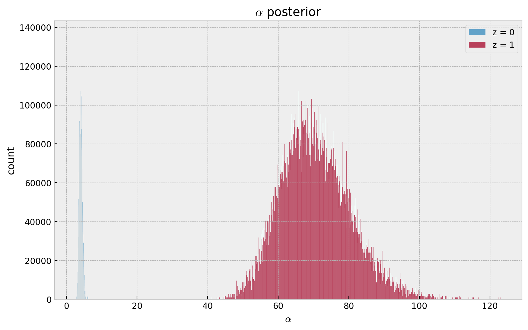
Effect in Parameters

• Recall \(\lambda \sim \text{Gamma}(r, \alpha)\), which has expected value \(r/\alpha\).
• As \(g_1 < 0\), then \(\alpha(z=1) > \alpha(z=0)\) which is consistent with the data generation process.

Hierarchical BG/NBD Model - Data

groups = ["g1", "g2", "g3", "g4"]

data_df["group"] = rng.choice(
    a=groups, p=[0.45, 0.35, 0.15, 0.05], size=n_obs
)

Hierarchical BG/NBD Model Structure

Hierarchical BG/NBD Model Results

Bayesian BG/NBD Model

It opens many posibilities and oportunities!

• Time-Invariant Covariates
• Hierarchical Models
• …

A sucessor package of lifetimes

Contributors needed!

References

Blog Posts

• BG/NBD Model in PyMC
• Gamma-Gamma Model of Monetary Value in PyMC

Papers

• Probability Models for Customer-Base Analysis
• Counting Your Customers: Who Are They and What Will They Do Next?
• “Counting Your Customers” the Easy Way: An Alternative to the Pareto/NBD Model
• Computing P(alive) Using the BG/NBD Model

Videos

• New Perspectives on CLV and E-Commerce Buying Patterns, Peter Fader

References

Software

Python

• lifetimes
• A sucessor package btyd of lifetimes.
• PyMC

R

• BTYD
• BTYDplus

Thank you!

juanitorduz.github.io