Gamma-Gamma Model of Monetary Value in PyMC

Prepare Notebook

import arviz as az
import matplotlib.pyplot as plt
import numpy as np
import seaborn as sns
from lifetimes.datasets import load_cdnow_summary_data_with_monetary_value
from lifetimes import GammaGammaFitter
import pymc3 as pm
import theano.tensor as tt

plt.style.use("bmh")
plt.rcParams["figure.figsize"] = [8, 6]
plt.rcParams["figure.dpi"] = 100

%load_ext autoreload
%autoreload 2
%config InlineBackend.figure_format = "svg"

Load Data

We are going to use an existing data set from the lifetimes package documentation, see here.

data_df = load_cdnow_summary_data_with_monetary_value()

data_df.info()

<class 'pandas.core.frame.DataFrame'>
Int64Index: 2357 entries, 1 to 2357
Data columns (total 4 columns):
 #   Column          Non-Null Count  Dtype  
---  ------          --------------  -----  
 0   frequency       2357 non-null   int64  
 1   recency         2357 non-null   float64
 2   T               2357 non-null   float64
 3   monetary_value  2357 non-null   float64
dtypes: float64(3), int64(1)
memory usage: 92.1 KB

From the package’s documentation:

• frequency: Number of repeat purchases the customer has made. More precisely, It’s the count of time periods the customer had a purchase in.
• monetary_value: represents the average value of a given customer’s purchases.

LEt us plot the distribution of the features of interest:

fig, ax = plt.subplots(
    nrows=1,
    ncols=2,
    figsize=(9, 4),
    sharex=False,
    sharey=False,
    layout="constrained"
)
sns.kdeplot(x="frequency", data=data_df, color="C2", clip=(0.0, None), fill=True, ax=ax[0])
ax[0].set(title="Frequency",xlabel="frequency (log)",xscale="log")
sns.kdeplot(x="monetary_value", data=data_df, color="C3", clip=(0.0, None), fill=True, ax=ax[1])
ax[1].set(title="Monetary Value",xlabel="monetary value (log)",xscale="log")
fig.suptitle("Data Distribution (log scale)", fontsize=16);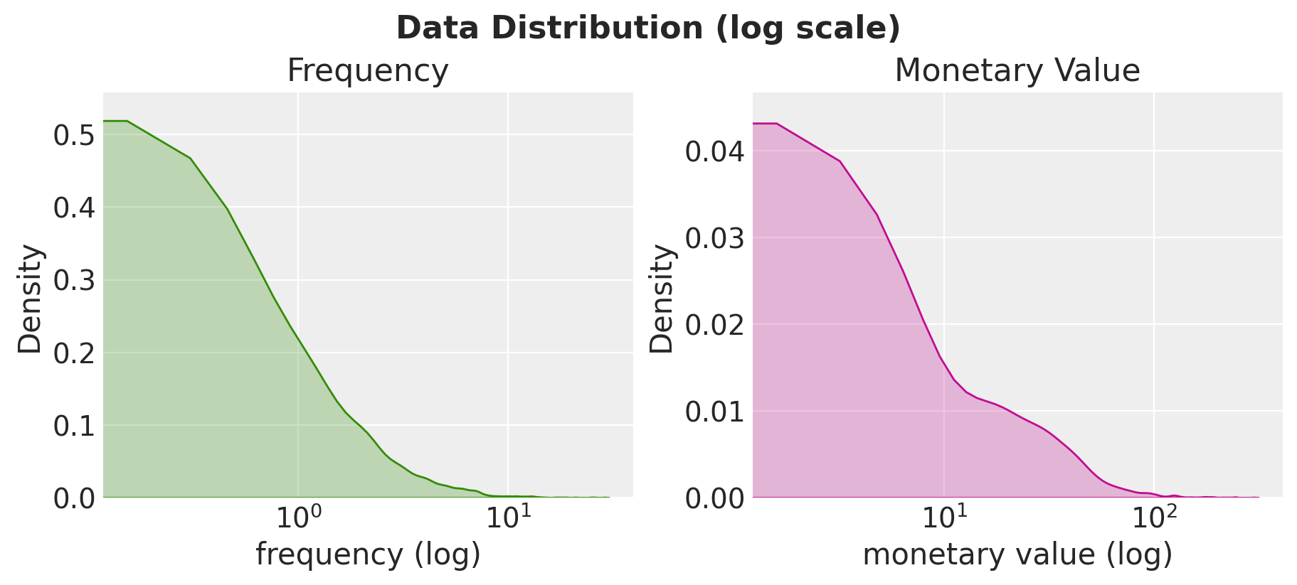

Gamma-Gamma Model (Lifetimes)

In this first section we we fit the model using the GammaGammaFitter class from the lifetimes package. Before fitting the model, let us recall the model specification (see “The Gamma-Gamma Model of Monetary Value”). First, here are the assumptions:

• The monetary value of a customer’s given transaction varies randomly around their average transaction value.
• Average transaction values vary across customers but do not vary over time for any given individual.
• The distribution of average transaction values across customers is independent of the transaction process.

Let \(\bar{z}\) be the observed average transaction value for a given customer. One is generally interested in the expected value \(E(Z|\bar{z}, x)\), where \(Z\) denotes the random variable of the customer monetary value per transaction and \(x\) is the observed frequency (see last section below). Now let us look into the concrete model parametrization:

• We assume that \(z_i \sim \text{Gamma}(p, \nu)\), with \(E(Z_i| p, \nu) = \xi = p/\nu\).
  • Given the convolution properties of the gamma, it follows that total spend across \(x\) transactions is distributed \(\text{Gamma}(px, \nu)\).
  • Given the scaling property of the gamma distribution, it follows \(\bar{z} \sim \text{Gamma}(px, νx)\).
• We assume \(\nu \sim \text{Gamma}(q, \gamma)\).

Remark: The notation used in the paper is slightly different from the one used in the lifetimes package. The parameter \(\gamma\) is denoted by \(v\).

For more details in the theory and the consequences of this parametrization please see the references above.

When fitting the model, we need to be careful with two conditions:

1. We must remove users without repeated purchases.
2. The Gamma-Gamma model assumes that there is no relationship between the monetary value and the purchase frequency.

For the first condition we simply filter out the data:

data_df.query("frequency > 0", inplace=True)

For the second condition we compute the correlation:

data_df.filter(["frequency", "monetary_value"]).corr()

	frequency	monetary_value
frequency	1.000000	0.113884
monetary_value	0.113884	1.000000

The correlation is not very high. Let us see it ins a scatter plot:

fig, ax = plt.subplots()
sns.scatterplot(x="frequency", y="monetary_value", data=data_df, ax=ax)
ax.set(title="Frequency vs Monetary Value",xlabel="frequency",ylabel="monetary value");

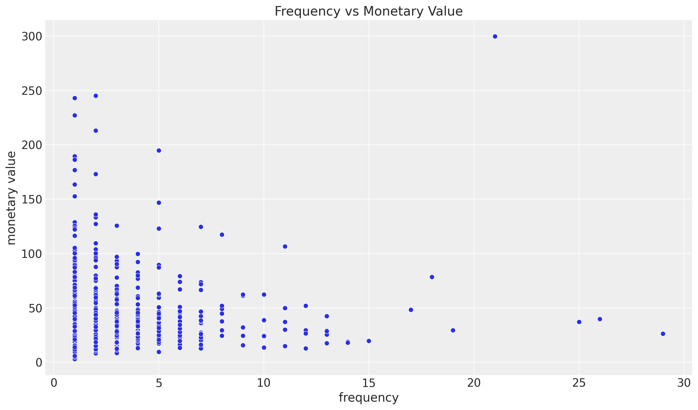
There does not seem to be a high relation between these features, so we can move and fir the lifetimes model.

# extract the data using the paper's (and lifetimes) notation 
x = data_df["frequency"].to_numpy()
m = data_df["monetary_value"].to_numpy()

ggf = GammaGammaFitter(penalizer_coef=0.0)
ggf.fit(frequency=x, monetary_value=m)

ggf.summary

	coef	se(coef)	lower 95% bound	upper 95% bound
p	6.248802	1.189687	3.917016	8.580589
q	3.744588	0.290166	3.175864	4.313313
v	15.447748	4.159994	7.294160	23.601336

These errors are computed using the Hessian (see for example here).

Bayesian Model

We use the same strategy of the post BG/NBD Model in PyMC where we rewrite the log-likelihood of the lifetimes package from numpy to theano. In this case the expression is much simpler, see the staticmethod of the class GammaGammaFitter._negative_log_likelihood.

with pm.Model() as model:

    p = pm.HalfNormal(name="p", sd=10)
    q = pm.HalfNormal(name="q", sd=10)
    v = pm.HalfNormal(name="v", sd=10)

    def logp(x, m):
        return (
            tt.gammaln(p * x + q)
            - tt.gammaln(p * x)
            - tt.gammaln(q)
            + q * tt.log(v)
            + (p * x - 1) * tt.log(m)
            + (p * x) * tt.log(x)
            - (p * x + q) * tt.log(x * m + v)
        )
    
    likelihood = pm.DensityDist(
        name="likelihood",
        logp=logp,
        observed = {"x":x, "m": m}
    )

Next, we estimate the posterior distribution.

with model:
    trace = pm.sample(
        tune=2000,
        draws=6000,
        chains=4,
        target_accept=0.95,
        return_inferencedata=True
    )

Let us take a look at the model summary:

az.summary(data=trace, var_names=["p", "q", "v"])

	mean	sd	hdi_3%	hdi_97%	mcse_mean	mcse_sd	ess_bulk	ess_tail	r_hat
p	6.991	1.352	4.733	9.541	0.018	0.013	5455.0	6269.0	1.0
q	3.663	0.257	3.198	4.150	0.003	0.002	5666.0	6580.0	1.0
v	14.021	3.466	7.963	20.688	0.049	0.035	5034.0	5506.0	1.0

We now plot the posterior distributions and compare them against the point estimate of the GammaFitter model.

axes = az.plot_trace(
    data=trace,
    lines=[(k, {}, [v]) for k, v in ggf.summary["coef"].items()],
    compact=True,
    backend_kwargs={
        "figsize": (10, 7),
        "layout": "constrained"
    },
)
fig = axes[0][0].get_figure()
fig.suptitle("Gamma-Gamma Model Trace");

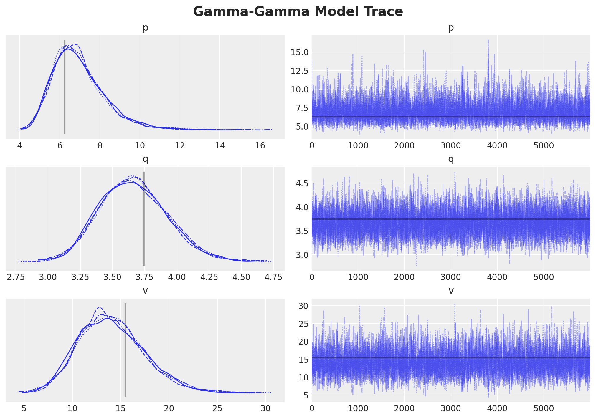
The results look comparable!

Finally, let’s look into the pair-plot of the posterior distributions:

axes = az.plot_pair(data=trace, var_names=["p", "q", "v"], figsize=(8, 8))
fig = plt.gcf()
fig.suptitle("Gamma-Gamma Model Parameters Pairplot", y=0.95, fontsize=16);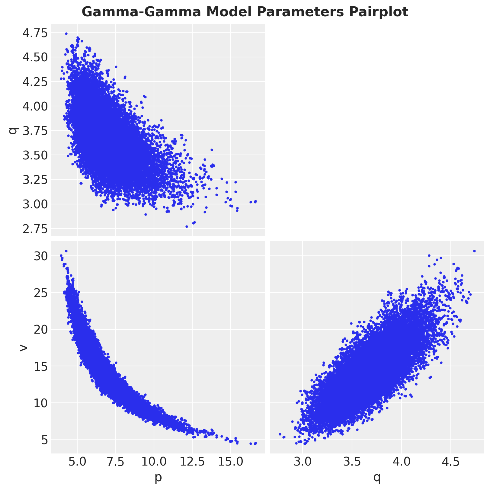

It is interesting to see that the p and v distributions seem to obey a non-linear relationship.

Conditional Expected Average Profit

Now that we have posterior samples at our disposal, we can compute quantities of interest using the expressions from the lifetimes package (and the papers of course). For example, let us compute the conditional expected average profit defined by the expected value \(E(Z|\bar{z}, x)\). One can show that the expected average profit is a weighted average of individual monetary value and the population mean (see Equation 5 in “The Gamma-Gamma Model of Monetary Value”).

First we compute it using the method GammaGammaFitter.conditional_expected_average_profit:

ggf_ceap = ggf.conditional_expected_average_profit(frequency=x, monetary_value=m)

Next, we compare it to the results from the pymc model. We do this by simply re-writing (specifically, vectorizing) the method above.

# pymc-examples/examples/time_series/Air_passengers-Prophet_with_Bayesian_workflow.html
def _sample(array, n_samples):
    """Little utility function, sample n_samples with replacement."""
    idx = np.random.choice(np.arange(len(array)), n_samples, replace=True)
    return array[idx]

def conditional_expected_average_profit(trace, x, m, n_samples):
    posterior = trace.posterior.stack(sample=('chain', 'draw'))
    p = _sample(array=posterior["p"], n_samples=n_samples).to_numpy()[..., None]
    q = _sample(array=posterior["q"], n_samples=n_samples).to_numpy()[..., None]
    v = _sample(array=posterior["v"], n_samples=n_samples).to_numpy()[..., None]

    individual_weight = p * x[None, ...] / (p * x[None, ...] + q - 1)
    population_mean = (v * p) / (q - 1)
    return (population_mean * (1 - individual_weight)) + (individual_weight * m)


n_samples = 1000

pymc_ceap = conditional_expected_average_profit(trace, x, m, n_samples)

Finally, we can compare the results:

fig, ax = plt.subplots(figsize=(8, 8))

ax.errorbar(
    x=ggf_ceap,
    y=pymc_ceap.mean(axis=0),
    yerr=az.hdi(ary=pymc_ceap).T,
    fmt="o",
    ecolor="C6",
    markeredgecolor="C1",
    markerfacecolor="C1",
    markersize=5,
    alpha=0.5,
    capsize=2,
)
ax.axline(
    xy1=(0, 0),
    slope=1,
    color="black",
    linestyle="--",
    label="diagonal"
)
ax.legend(loc="upper left")
ax.set(title="Model Comparison", xlabel="lifetimes", ylabel="pymc");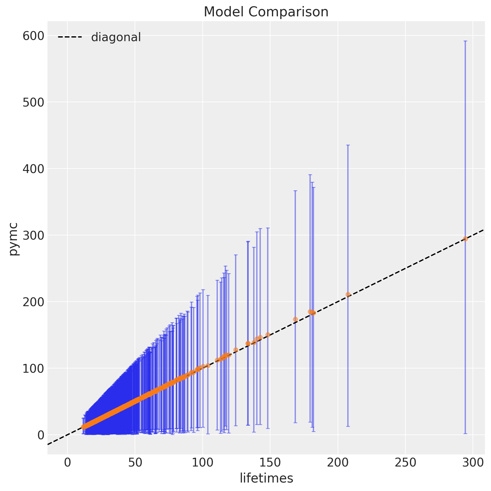

Note that the credible intervals increase as the monetary value increases. This is no surprise given the data distribution (see first plot above).

Remark: Note that the credible intervals are always positive:

assert az.hdi(ary=pymc_ceap).min().min() > 0