%%{init: {"theme": "white", "themeVariables": {"fontSize": "48px"}, "flowchart":{"htmlLabels":false}}}%%
flowchart TD
N[Number of Users] --> N_active[Number of Active Users]
N_active --> Retention[Retention]
Retention --> Revenue[Revenue]
Cohort Revenue & Retention Analysis: A Bayesian Approach
PyData Berlin - July 2023
Mathematician & Data Scientist
Outline
Introduction
Bottom-Up Approaches
2.1 Shifted Beta Geometric (Contractual)
2.2 BG/NBD Model (Non-Contractual)
Simple Cohort Retention Model (GLM)
Retention Model with BART
Cohort Revenue-Retention Model
Applications
References
Business Problem
Example
During January \(2020\), \(100\) users signed up for a service (cohort).
In February \(2020\), there were \(17\) users from the \(2020-01\) cohort active (e.g. did at least one purchase). The retention rate is \(17\%\).
We want to understand and predict how retention develops over time.
The main motivation is to estimate customer lifetime value (CLV).
Number of Active Users
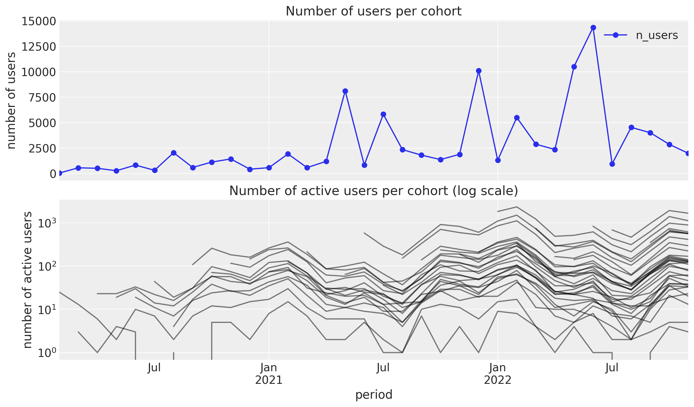
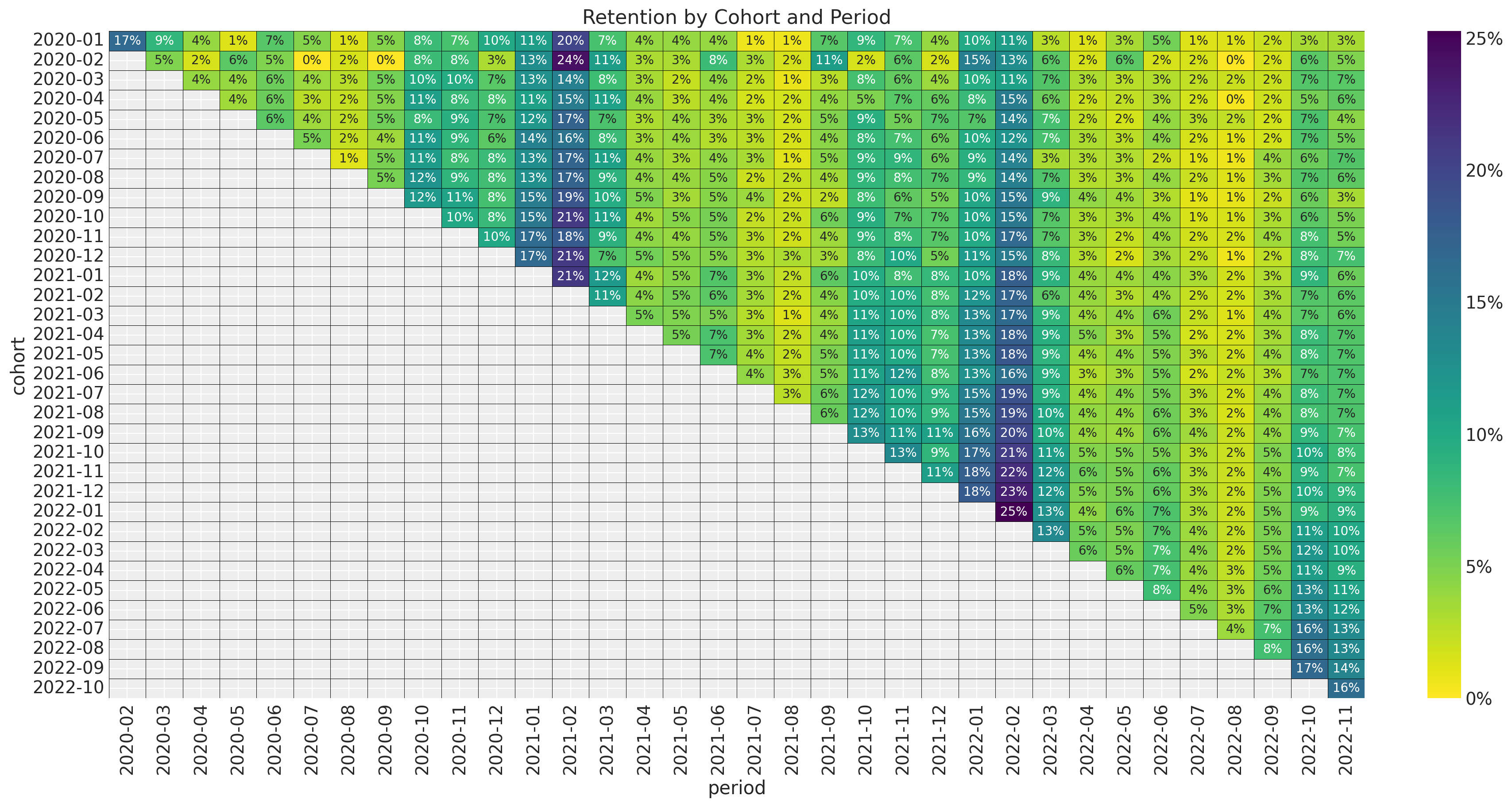
Retention Matrix
Bottom-Up Approaches
Predict the retention of each user individually and then aggregate the results.
Example: Shifted Beta Geometric (Contractual)
An individual remains a customer of the company with constant retention probability \(1 - \theta\). This is equivalent to assuming that the duration of the customer’s relationship with the company, denoted by the random variable \(T\), is characterized by the (shifted) geometric distribution with probability mass function and survivor function given by
\[f(T=t|\theta) = \theta (1 - \theta)^{t - 1}, \quad t = 1, 2, \ldots\]
\[S(t) = \sum_{j = t}^{\infty} f(T=j|\theta) = (1 - \theta)^{t}, \quad t = 1, 2, \ldots\]
Heterogeneity in \(\theta\) follows a beta distribution \(\theta \sim \text{Beta}(a, b)\).
Shifted Beta Geometric - Survival Function
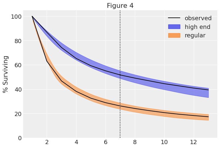
See pymc-marketing example here.
Bottom-Up Approaches
Example: BG/NBD Model (Non-Contractual)
While active, the time between transactions is distributed exponentially with transaction rate, i.e.,
\[f(t_{j}|t_{j-1}; \lambda) = \lambda \exp(-\lambda (t_{j} - t_{j - 1})), \quad t_{j} \geq t_{j - 1} \geq 0\]
Heterogeneity in \(\lambda\) follows a gamma distribution \(\lambda \sim \text{Gamma}(r, \alpha)\).
After any transaction, a customer becomes inactive with probability \(p\).
Heterogeneity in \(p\) follows a beta distribution \(p \sim \text{Beta}(a, b)\).
The transaction rate \(\lambda\) and the dropout probability \(p\) vary independently across customers.
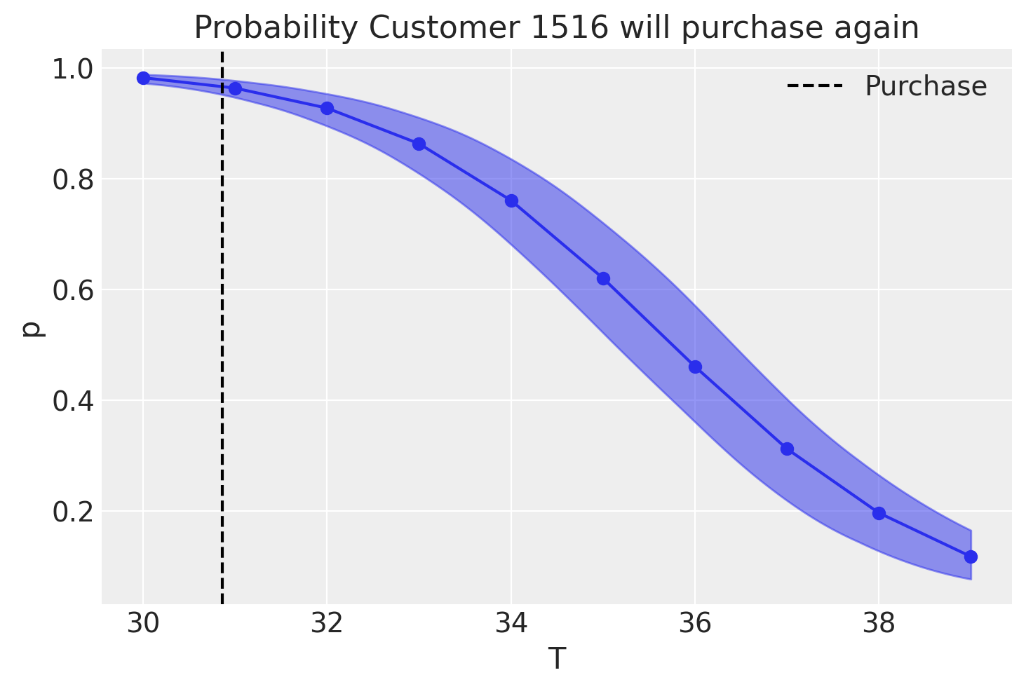
BG/NBD - Probability of Alive
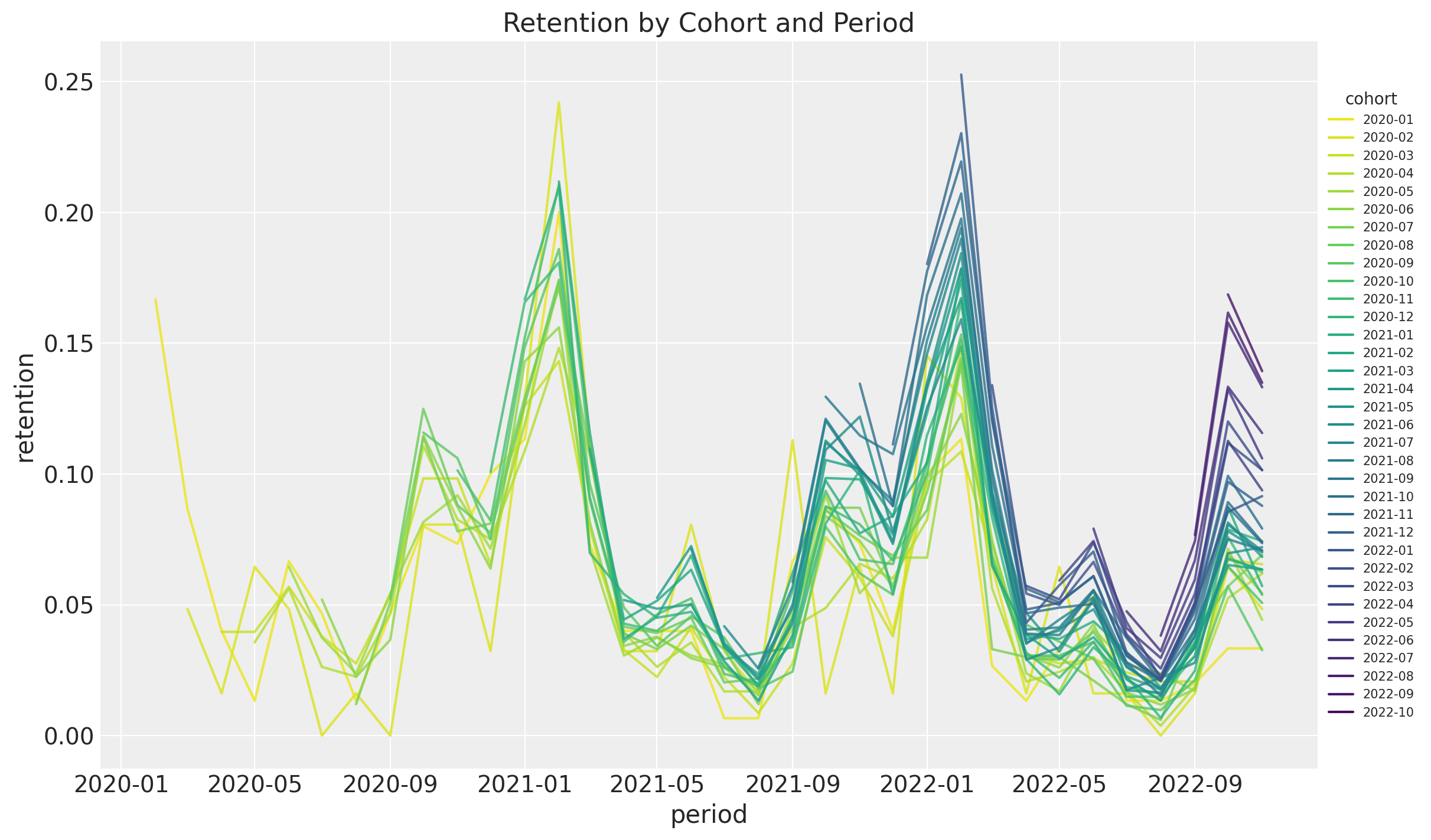
Retention Matrix
- Cohort Age: Age of the cohort in months.
- Age: Age of the cohort with respect to the observation time.
- Month: Month of the observation time (period).
Retention Over Time (period)
Retention - Generalized Linear Model
\[\begin{align*} N_{\text{active}} \sim & \: \text{Binomial}(N_{\text{total}}, p) \\ \textrm{logit}(p) = & \: ( \text{intercept} \\ & + \beta_{\text{cohort age}} \text{cohort age} \\ & + \beta_{\text{age}} \text{age} \\ & + \beta_{\text{cohort age} \times \text{age}} \text{cohort age} \times \text{age} \\ & + \beta_{\text{seasonality}} \text{seasonality} ) \end{align*}\]
where \(p\) represents the retention and \(\text{logit}: (0, 1) \longrightarrow \mathbb{R}\) is defined by \(\text{logit}(p) = \log\left(\frac{p}{1-p}\right)\).
Retention - GLM in PyMC

Retention - GLM in PyMC
with pm.Model(coords=coords) as model:
    # --- Data ---
    model.add_coord(name="obs", values=train_obs_idx, mutable=True)
    age_scaled = pm.MutableData(
        name="age_scaled", value=train_age_scaled, dims="obs"
    )
    cohort_age_scaled = pm.MutableData(
        name="cohort_age_scaled", value=train_cohort_age_scaled, dims="obs"
    )
    period_month_idx = pm.MutableData(
        name="period_month_idx", value=train_period_month_idx, dims="obs"
    )
    n_users = pm.MutableData(
        name="n_users", value=train_n_users, dims="obs"
    )
    n_active_users = pm.MutableData(
        name="n_active_users", value=train_n_active_users, dims="obs"
    )

    # --- Priors ---
    intercept = pm.Normal(name="intercept", mu=0, sigma=1)
    b_age_scaled = pm.Normal(name="b_age_scaled", mu=0, sigma=1)
    b_cohort_age_scaled = pm.Normal(
        name="b_cohort_age_scaled", mu=0, sigma=1
    )
    b_period_month = pm.ZeroSumNormal(
        name="b_period_month", sigma=1, dims="period_month"
    )
    b_age_cohort_age_interaction = pm.Normal(
        name="b_age_cohort_age_interaction", mu=0, sigma=1
    )

    # --- Parametrization ---
    mu = pm.Deterministic(
        name="mu",
        var=intercept
        + b_age_scaled * age_scaled
        + b_cohort_age_scaled * cohort_age_scaled
        + b_age_cohort_age_interaction * age_scaled * cohort_age_scaled
        + b_period_month[period_month_idx],
        dims="obs",
    )

    p = pm.Deterministic(name="p", var=pm.math.invlogit(mu), dims="obs")

    # --- Likelihood ---
    pm.Binomial(
        name="likelihood",
        n=n_users,
        p=p,
        observed=n_active_users,
        dims="obs",
)Posterior Distribution
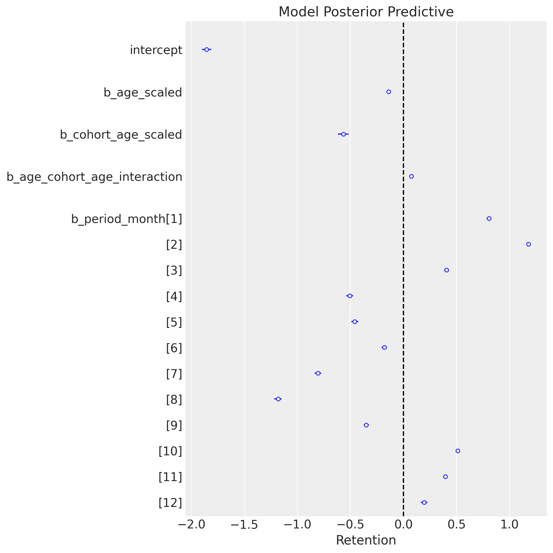
Posterior Predictive Check
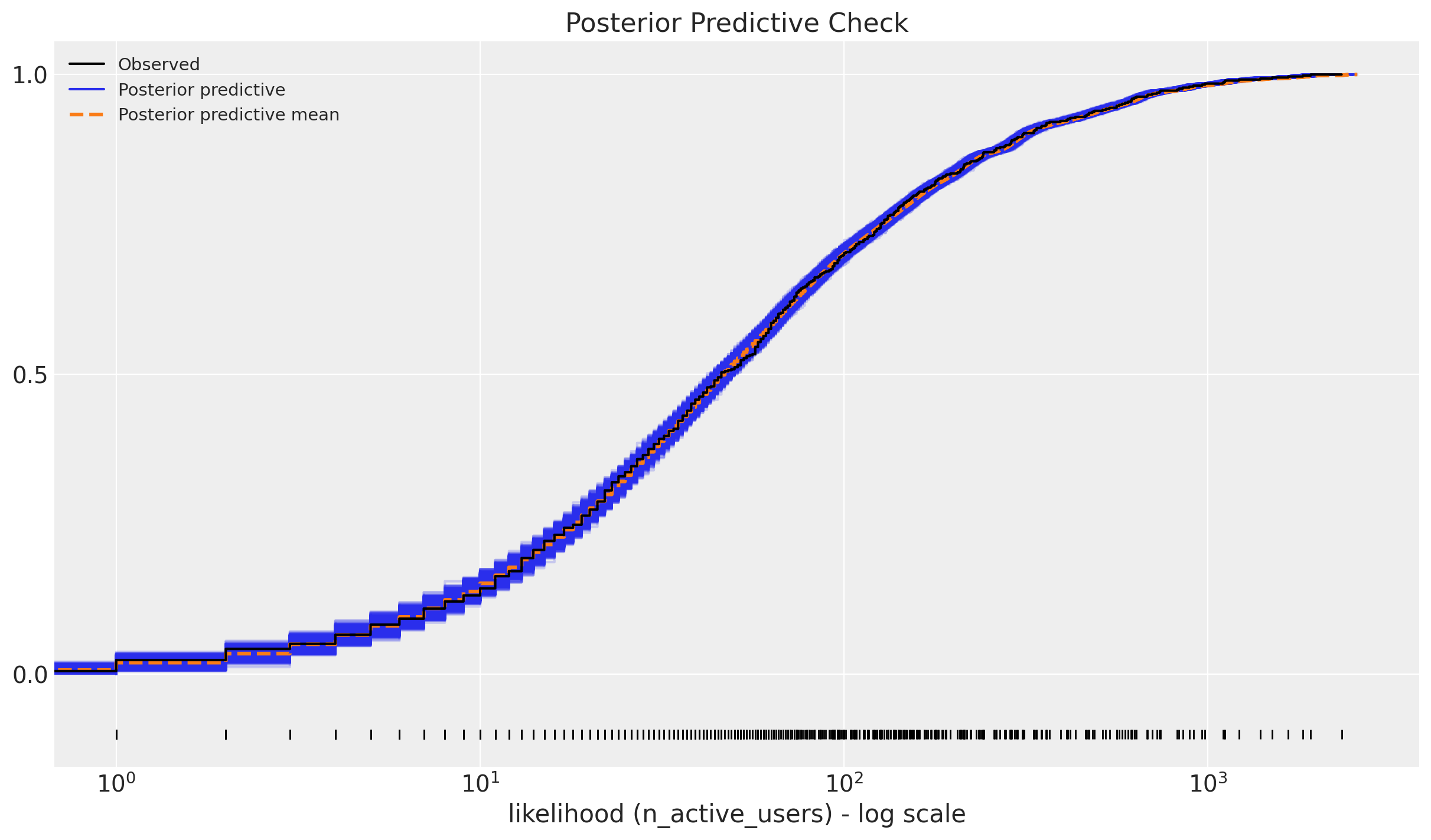
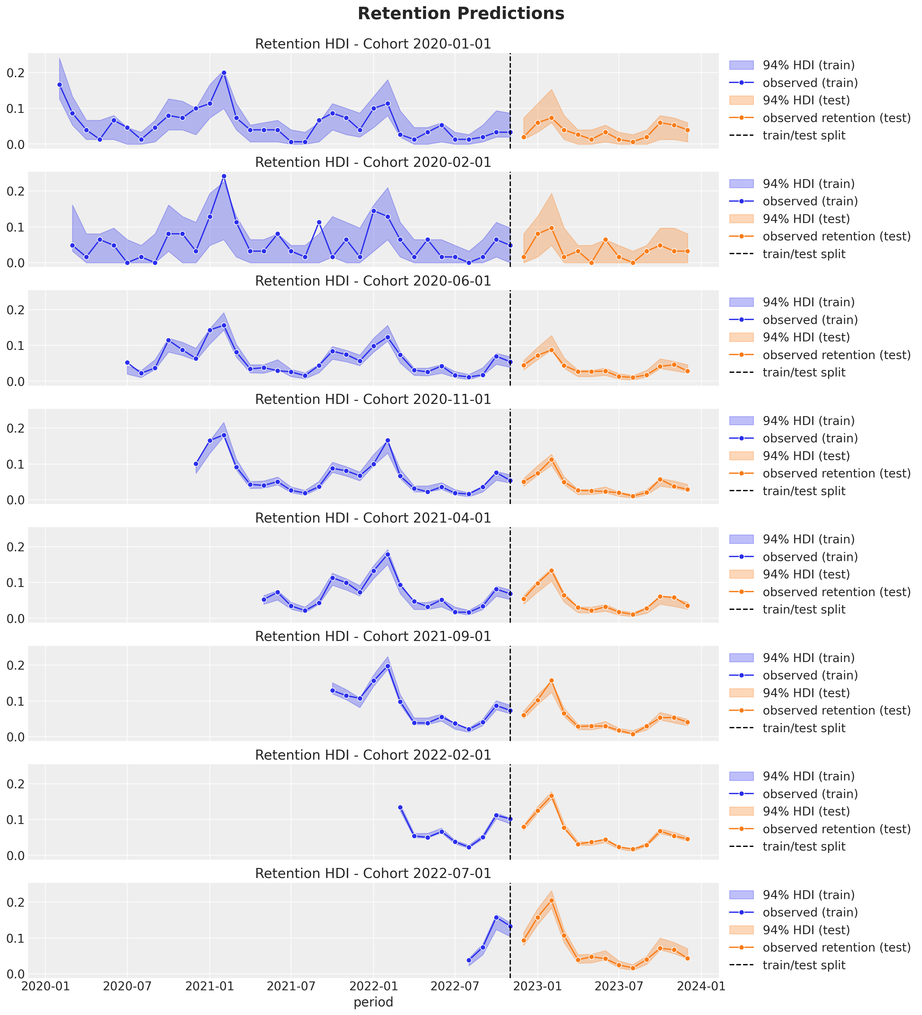
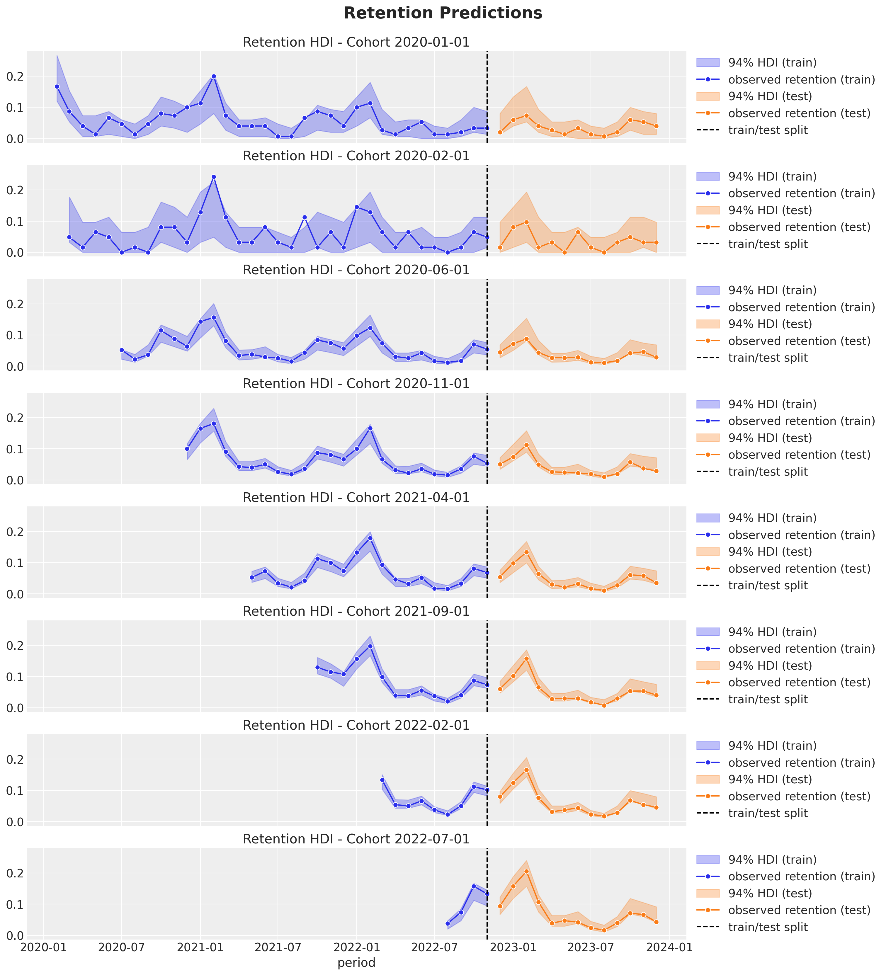
In-Sample Predictions
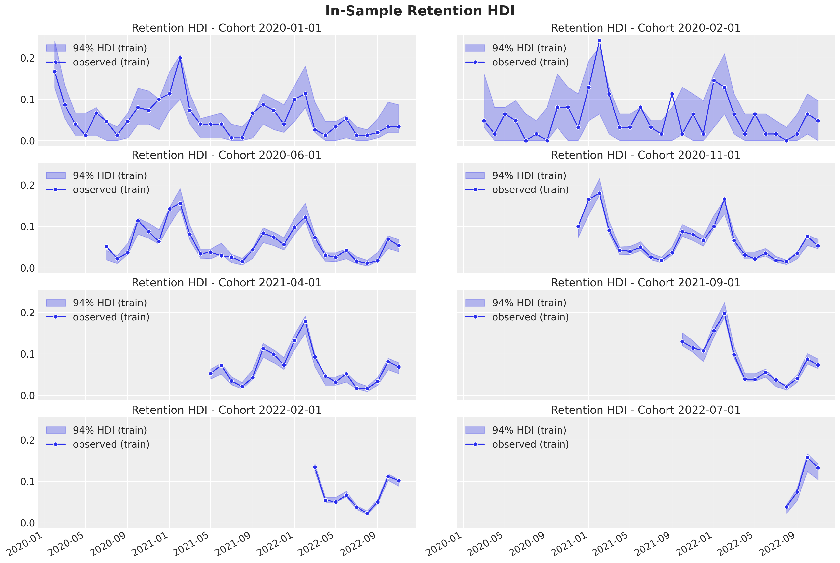
Out-of-Sample Predictions
More Complex Models - Requirements
In many real-world scenarios, the data is more complex and the linear model is not enough. We need a more flexible model that can capture non-linearities and interactions.
We care about uncertainty.
We want to be able to iterate fast.
Interested in out-of-sample predictions.
We want to couple retention modeling with revenue modeling (CLV).
Bayesian Additive Regression Trees
Bayesian “sum-of-trees” model where each tree is constrained by a regularization prior to be a weak learner.
To fit the sum-of-trees model, BART uses PGBART, an inference algorithm based on the particle Gibbs method.
BART depends on the number of trees \(m\in \mathbb{N}\) and prior parameters \(\alpha \in (0, 1)\) and \(\beta \in [0, \infty)\) so that the probability that a node at depth \(d \in \mathbb{N}_{0}\) is nonterminal is \(\alpha(1 + d)^{-\beta}\).
BART is implemented in
pymc-bart.
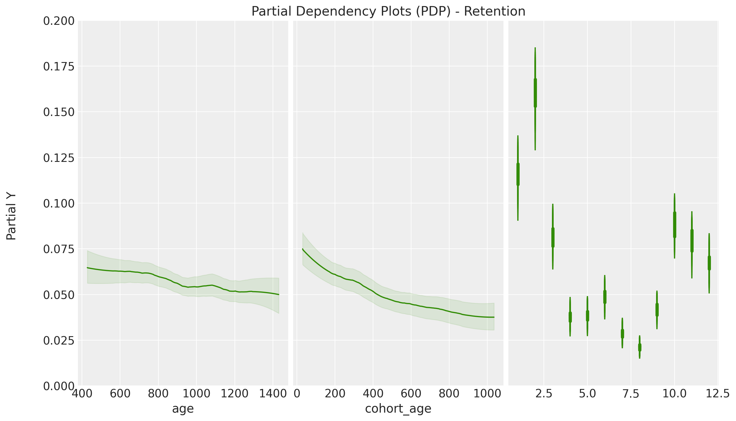
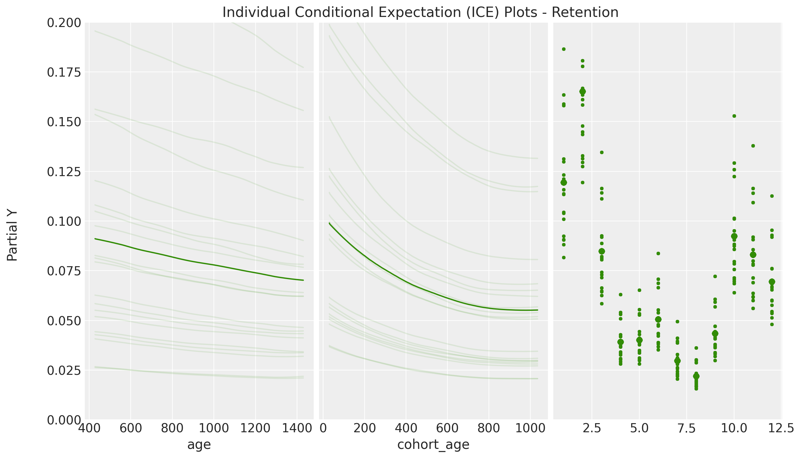
BART Retention Model
\[\begin{align*} N_{\text{active}} & \sim \text{Binomial}(N_{\text{total}}, p) \\ \textrm{logit}(p) & = \text{BART}(\text{cohort age}, \text{age}, \text{month}) \end{align*}\]

PDP Plot
ICE Plot
Revenue
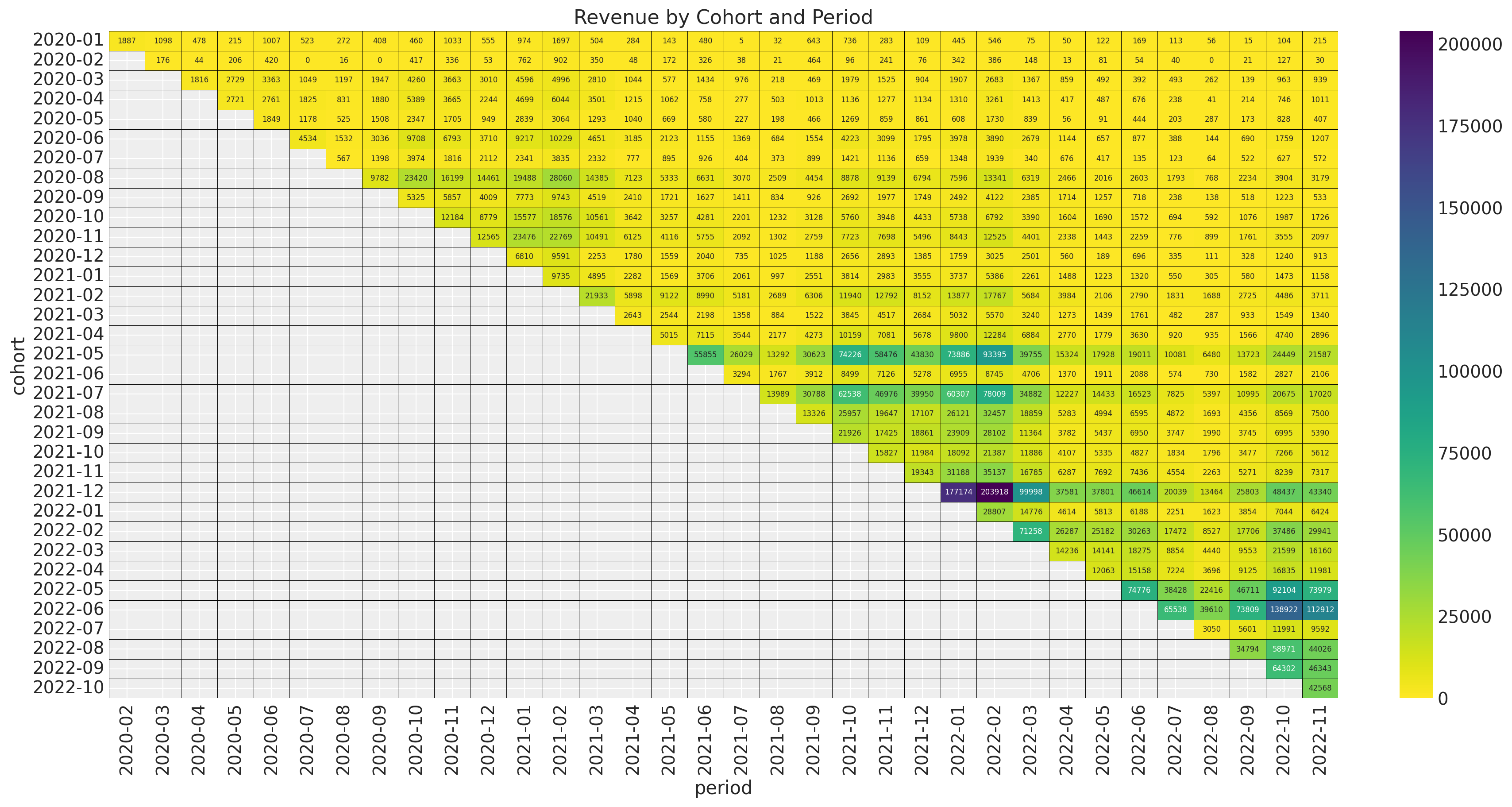
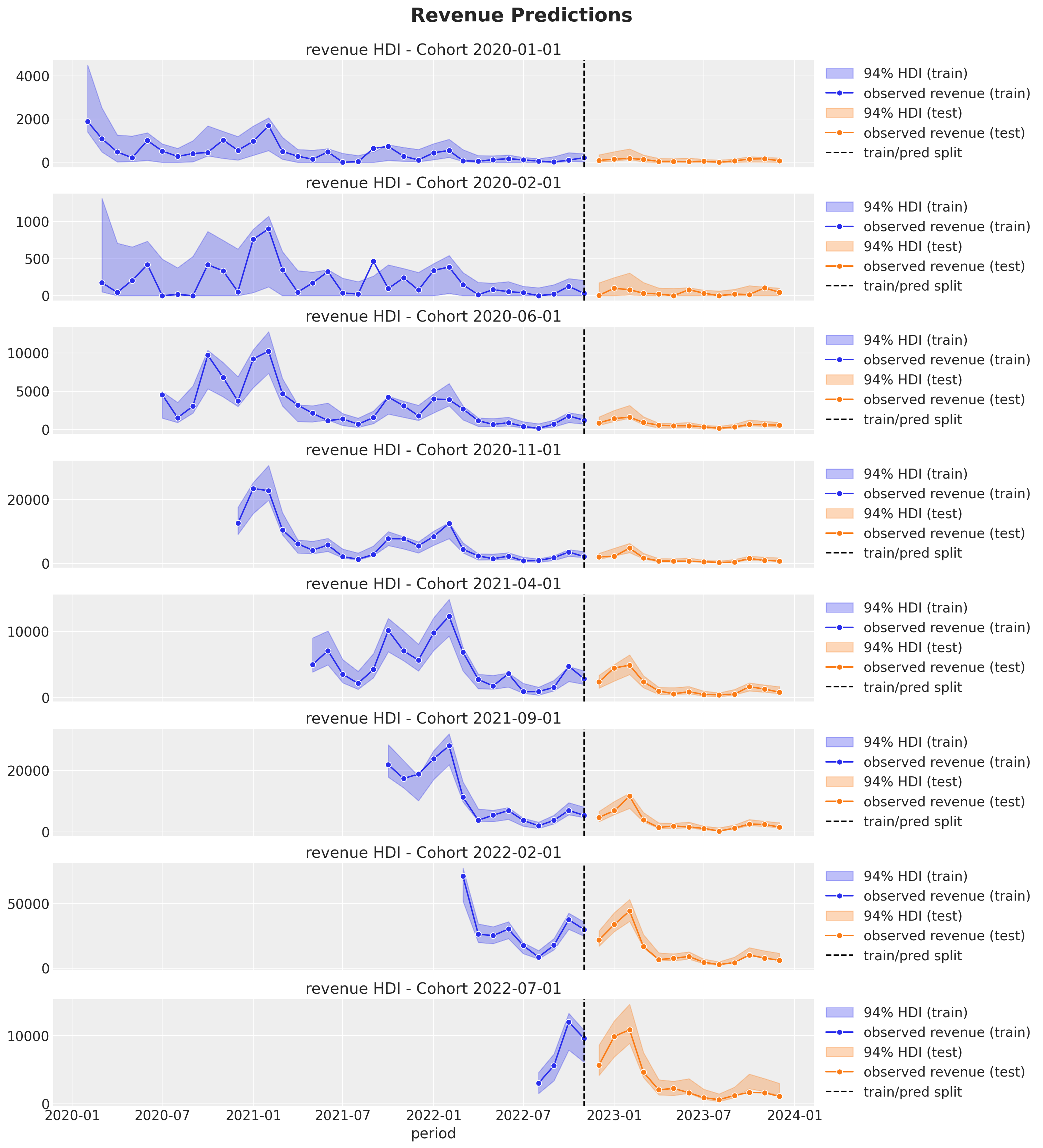
Cohort Revenue-Retention Model
Retention Component
\[\begin{align*} \textrm{logit}(p) & = \text{BART}(\text{cohort age}, \text{age}, \text{month}) \\ N_{\text{active}} & \sim \text{Binomial}(N_{\text{total}}, p) \end{align*}\]
Revenue Component
\[\begin{align*} \log(\lambda) = \: (& \text{intercept} \\ & + \beta_{\text{cohort age}} \text{cohort age} \\ & + \beta_{\text{age}} \text{age} \\ & + \beta_{\text{cohort age} \times \text{age}} \text{cohort age} \times \text{age}) \\ \text{Revenue} & \sim \text{Gamma}(N_{\text{active}}, \lambda) \end{align*}\]
Cohot Revenue-Retention Model
mu = pmb.BART(
    name="mu", X=x, Y=train_retention_logit, m=100, response="mix", dims="obs"
)

p = pm.Deterministic(name="p", var=pm.math.invlogit(mu), dims="obs")

lam_log = pm.Deterministic(
    name="lam_log",
    var=intercept
    + b_age_scaled * age_scaled
    + b_cohort_age_scaled * cohort_age_scaled
    + b_age_cohort_age_interaction * age_scaled * cohort_age_scaled,
    dims="obs",
)

lam = pm.Deterministic(name="lam", var=pm.math.exp(lam_log), dims="obs")

n_active_users_estimated = pm.Binomial(
    name="n_active_users_estimated",
    n=n_users,
    p=p,
    observed=n_active_users,
    dims="obs",
)

x = pm.Gamma(
    name="revenue_estimated",
    alpha=n_active_users_estimated + eps,
    beta=lam,
    observed=revenue,
    dims="obs",
)
Cohort Revenue-Retention Model

Revenue-Retention - Predictions
Some Applications in the Industry
Understand retention and revenue drivers.
Factor out seasonality.
External covariates (e.g. acquisition channel).
Forecast revenue and retention (cohort lifetime value).
Causal Inference
Counterfactural analysis.
Geo experiments.
References
Blog Posts
Packages
Papers
- BART: Bayesian additive regression trees
- Bayesian additive regression trees for probabilistic programming
References
Related Work
“Counting Your Customers” the Easy Way: An Alternative to the Pareto/NBD Model, see
pymc-marketingexample here.How to Project Customer Retention, see
pymc-marketingexample here.
Open Source Packages

Thank you!

![]()