Introduction to Bayesian Modeling with PyMC

PyCon Colombia 2022

Dr. Juan Orduz

Why Bayesian Modeling?

• Conceptually transparent interpretation of probablity.
• Uncertainty quantification.
• Allows to explicitly include prior knowledge in the model.
• Felxible and suited for many applications in academia and industry.
• Scalable*

Why PyMC?

Bayesian Inference : An Example

Suppose you see a person with long hair. You want to estimate the probablity that this person is a woman. That is, for \(A = \text{woman}\) and \(B = \text{long hair}\), we want to estimate \(P(A|B)\)

Prior-Information

You belive \(P(A) = 0.5\), \(P(B)=0.4\) and \(P(B|A) = 0.7\).

Bayes Rule

\[ P(A|B) = \frac{P(A)\times P(B|A)}{P(B)} = \frac{0.5 \times 0.7}{0.4} = 0.875 \]

Some Examples: Distributions

Bayesian Approach to Data Analysis

Assume \(y\sim p(y|\theta)\), where \(\theta\) is a parameter(s) for the distribution (e.g. \(y\sim N(\mu, \sigma^2)\)). From Bayes Theorem:

\[ p(\theta|y)=\frac{p(y|\theta) \times p(\theta)}{p(y)} = \displaystyle{\frac{p(y|\theta)\times p(\theta)}{\color{red}{\int p(y|\theta)p(\theta)d\theta}}} \]

• The function \(p(y|\theta)\) is called the likelihood.
• \(p(\theta)\) is the prior distribution of \(\theta\).

\[ p(\theta|y) \propto \text{likelihood} \times \text{prior}. \]

Integrals are hard to compute \(\Longrightarrow\) we need samplers.

Example : Linear Regression

\[\begin{align*} y & \sim \text{Normal}(\mu, \sigma^2)\\ \mu & = a + bx \end{align*}\]

Objective: We want to estimate the (posterior) distributions of \(a\), \(b\) (and hence \(\mu\)) and \(\sigma\) given \(x\) and \(y\).

Example : Linear Regression

Model Specification: Math

Model Parametrization: \[\begin{align*} y & \sim \text{Normal}(\mu, \sigma^2)\\ \mu & = a + bx \\ \end{align*}\]

Prior Distributions: \[\begin{align*} a & \sim \text{Normal}(0, 2)\\ b & \sim \text{Normal}(0, 2) \\ \sigma & \sim \text{HalfNormal}(2) \end{align*}\]

Model Specification: PyMC

with pm.Model(coords={"idx": range(n_train)}) as model:

    # --- Data Containers ---
    x = pm.MutableData(name="x", value=x_train)
    y = pm.MutableData(name="y", value=y_train)
    
    # --- Priors ---
    a = pm.Normal(name="a", mu=0, sigma=2)
    b = pm.Normal(name="b", mu=0, sigma=2)
    sigma = pm.HalfNormal(name="sigma", sigma=2)
    
    # --- Model Parametrization ---
    mu = pm.Deterministic(name="mu", var=a + b * x, dims="idx")
    
    # --- Likelihood ---
    likelihood = pm.Normal(
        name="likelihood", mu=mu, sigma=sigma, observed=y, dims="idx"
    )

Compare to:

sklearn.linear_model.LinearRegression

Prior Predictive Sampling

with model:
    prior_predictive = pm.sample_prior_predictive(samples=100)

Prior samples before passing the data through the model.

Fit Model

with model:
    idata = pm.sample(target_accept=0.8, draws=1_000, chains=4)
    posterior_predictive = pm.sample_posterior_predictive(trace=idata)

Posterior samples distriibution via NUTS sampler in PyMC. For each parameter we run 4 iindependent chains with 1000 samples each.

Posterior Predictive (Training Set)

Posterior distribution of \(\mu\).

Posterior distribution of \(y\).

Posterior Predictive (Test Set)

Posterior distribution of \(\mu\).

Posterior distribution of \(y\).

Model Variations: Prior Constraints

with pm.Model(coords={"idx": range(n_train)}) as model:
    
    # --- Data Containers ---
    x = pm.MutableData(name="x", value=x_train)
    y = pm.MutableData(name="y", value=y_train)
    
    # --- Priors ---
    a = pm.Normal(name="a", mu=0, sigma=2)
    b = pm.HalfNormal(name="b", sigma=2)
    sigma = pm.HalfNormal(name="sigma", sigma=2)
    
    # --- Model Parametrization ---
    mu = pm.Deterministic(name="mu", var=a + b * x, dims="idx")
    
    # --- Likelihood ---
    likelihood = pm.Normal(
        name="likelihood", mu=mu, sigma=sigma, observed=y, dims="idx"
    )

Compare to:

sklearn.linear_model.LinearRegression with positive = True.

Model Variations: Regularization

with pm.Model(coords={"idx": range(n_train)}) as model:
    
    # --- Data Containers ---
    x = pm.MutableData(name="x", value=x_train)
    y = pm.MutableData(name="y", value=y_train)
    
    # --- Priors ---
    a = pm.Normal(name="a", mu=0, sigma=2)
    b = pm.Laplace(name="b", sigma=2)
    sigma = pm.HalfNormal(name="sigma", sigma=2)
    
    # --- Model Parametrization ---
    mu = pm.Deterministic(name="mu", var=a + b * x, dims="idx")
    
    # --- Likelihood ---
    likelihood = pm.Normal(
        name="likelihood", mu=mu, sigma=sigma, observed=y, dims="idx"
    )

Compare to:

sklearn.linear_model.Ridge

Model Variations: Robust Regression

with pm.Model(coords={"idx": range(n_train)}) as model:
    
    # --- Data Containers ---
    x = pm.MutableData(name="x", value=x_train)
    y = pm.MutableData(name="y", value=y_train)
    
    # --- Priors ---
    a = pm.Normal(name="a", mu=0, sigma=2)
    b = pm.Normal(name="b", mu=0, sigma=2)
    sigma = pm.HalfNormal(name="sigma", sigma=2)
    nu = pm.Gamma(name="nu", a=10, b=10)
    
    # --- Model Parametrization ---
    mu = pm.Deterministic(name="mu", var=a + b * x, dims="idx")
    
    # --- Likelihood ---
    likelihood = pm.StudentT(
        name="likelihood", mu=mu, sigma=sigma, nu=nu, observed=y, dims="idx"
    )

Compare to:

sklearn.linear_model.HuberRegressor

Example: Bike Rental Model

Example: Bike Rental Model

Linear Regression Baseline

\[ \text{cnt} = \text{intercept} + b_{\text{temp}}\text{temp} + \cdots \]

Example: Bike Rental Model

Linear Regression Baseline

Example: Bike Rental Model

Two ML Models: Linear Regression (\(L^1\)) with second order interactions and XGBoost

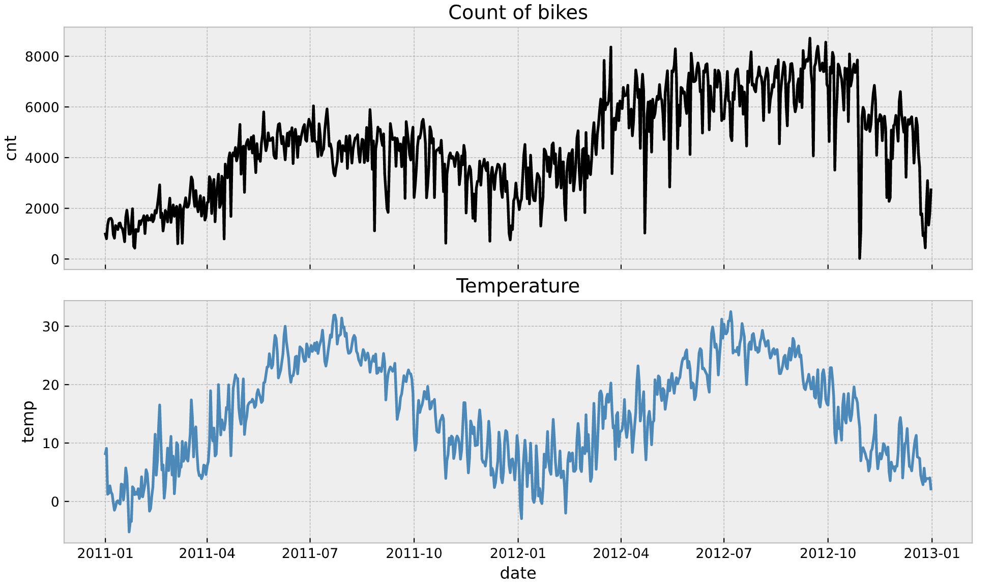
Example: Bike Rental Model

Two ML Models: Both see a negative effect of temperature in bke rentals ini the month of July.

Example: Bike Rental Model

Time-Varying Coefficients

\[ b(t) \sim N(b(t - 1), \sigma^2) \]

Example: Bike Rental Model

Time-Varying Coefficients

Example: Bike Rental Model

Time-Varying Coefficients

Example: Bike Rental Model

Time-Varying Coefficients

Effect of temperature on bike rentals as a function of tmie for a time varying coeffiicient model (via Gaussian random walk).

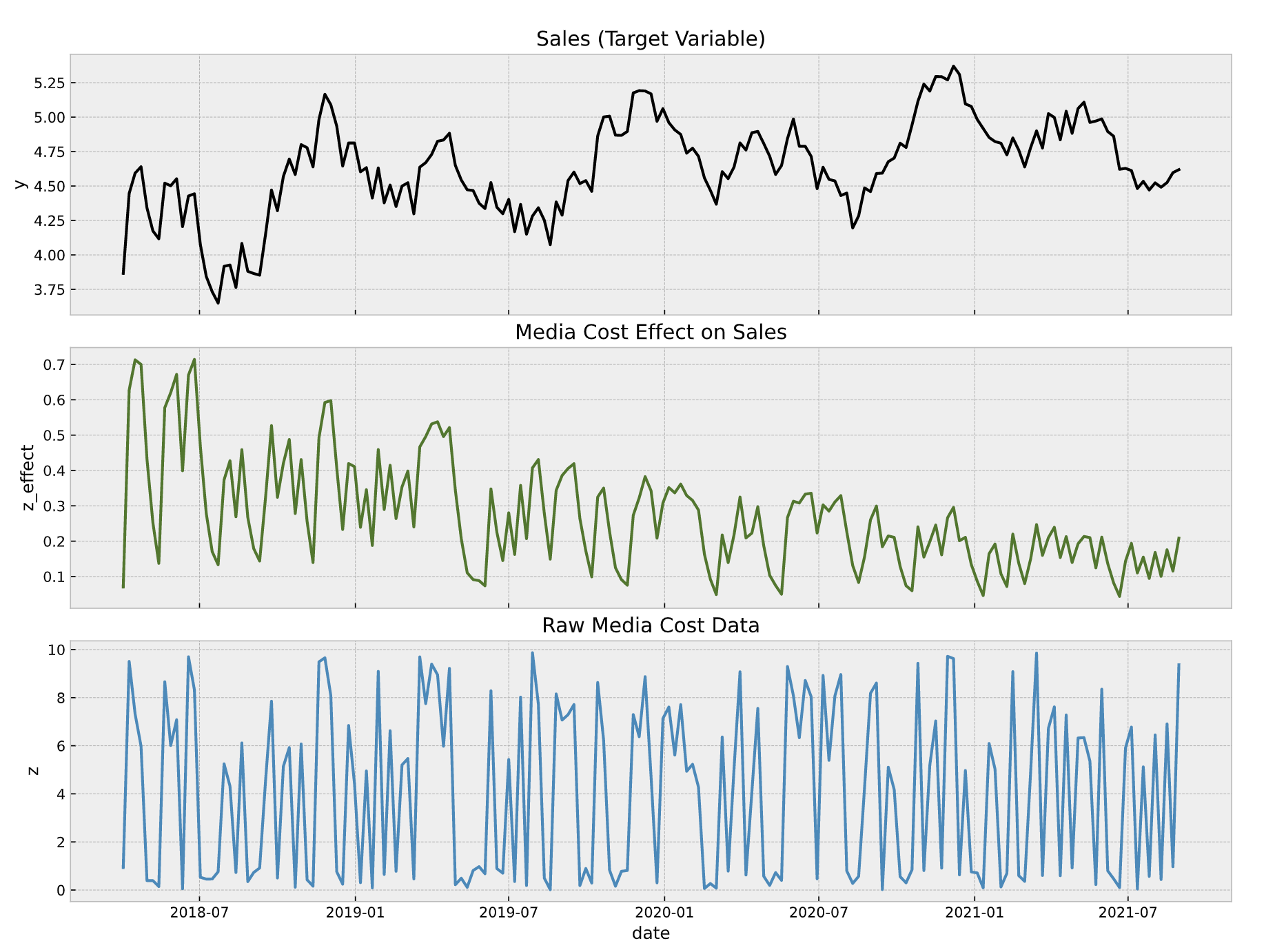
Application: Media Mix Model (MMM)

Application: Media Mix Model (MMM)

MMM structure: Media data (cost, impressions or clicks) is modeled using carryover effects (adstock) and saturation effects. In addition, one can control for seasonality and external regressors. In this example, we allow time-varying coefficients to capture the effect development over time.

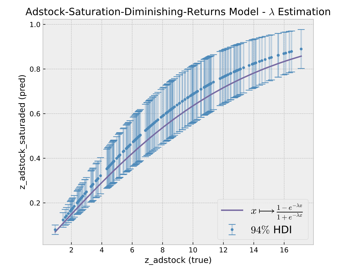
Application: Media Mix Model (MMM)

Fitted saturation effect. This can be used for media mix budget optimization.

Estimated effect varying over time.

Many More Examples and Applications!

References

Theory

• Statistical Rethinking by Richard McElreath
  • Statistical Rethinking in PyMC

PyMC

• PyMC Documentation: Example Gallery

• Online Book: Bayesian Modeling and Computation in Python

Use cases

• https://learnbayesstats.com/

Thank you!

juanitorduz.github.io