In this notebook we want to illustrate how to use PyMC to fit a time-varying coefficient regression model. The motivation comes from post Exploring Tools for Interpretable Machine Learning where we studied a time series problem, regarding the prediction of the number of bike rentals, from a machine learning perspective. Concretely, we fitted and compared two machine learning models: a linear regression with interactions and a gradient boost model (XGBoost). The models regressors were mainly meteorological data and seasonality features. One interesting feature we saw, through PDP and ICE plots was that the temperature feature had a non-constant effect over the bike rentals (see here). Indeed, when the temperature is high (more than 25 degrees approximately), the bike rentals are negatively impacted by the temperature (to be fair, this is when controlling by other regressors) on average. What we want to do in this notebook is to tackle the same problem from a different perspective. Namely, use to use a GaussianRandomWalk to model the interaction effect between the temperature and the bike rentals. We of course start with the simple regression baseline for comparison.
Prepare Notebook
import arviz as az
import matplotlib.pyplot as plt
import numpy as np
import pandas as pd
import pymc as pm
from pymc.distributions.continuous import Exponential
from sklearn.preprocessing import MinMaxScaler
import seaborn as sns


plt.style.use("bmh")
plt.rcParams["figure.figsize"] = [10, 6]
plt.rcParams["figure.dpi"] = 100
plt.rcParams["figure.facecolor"] = "white"

%load_ext autoreload
%autoreload 2
%config InlineBackend.figure_format = "retina"
seed: int = sum(map(ord, "bikes"))
rng: np.random.Generator = np.random.default_rng(seed=seed)Read Data
For a detailed description of the data set please see here (from the book Interpretable Machine Learning:A Guide for Making Black Box Models Explainable by Christoph Molnar). For a detailed EDA see the previous post Exploring Tools for Interpretable Machine Learning.
data_path = "https://raw.githubusercontent.com/christophM/interpretable-ml-book/master/data/bike.csv"

raw_data_df = pd.read_csv(
    data_path,
    dtype={
        "season": "category",
        "mnth": "category",
        "holiday": "category",
        "weekday": "category",
        "workingday": "category",
        "weathersit": "category",
        "cnt": "int",
    },
)

raw_data_df.head()
| season | yr | mnth | holiday | weekday | workingday | weathersit | temp | hum | windspeed | cnt | days_since_2011 | |
|---|---|---|---|---|---|---|---|---|---|---|---|---|
| 0 | WINTER | 2011 | JAN | NO HOLIDAY | SAT | NO WORKING DAY | MISTY | 8.175849 | 80.5833 | 10.749882 | 985 | 0 |
| 1 | WINTER | 2011 | JAN | NO HOLIDAY | SUN | NO WORKING DAY | MISTY | 9.083466 | 69.6087 | 16.652113 | 801 | 1 |
| 2 | WINTER | 2011 | JAN | NO HOLIDAY | MON | WORKING DAY | GOOD | 1.229108 | 43.7273 | 16.636703 | 1349 | 2 |
| 3 | WINTER | 2011 | JAN | NO HOLIDAY | TUE | WORKING DAY | GOOD | 1.400000 | 59.0435 | 10.739832 | 1562 | 3 |
| 4 | WINTER | 2011 | JAN | NO HOLIDAY | WED | WORKING DAY | GOOD | 2.666979 | 43.6957 | 12.522300 | 1600 | 4 |
Data Formatting
data_df = raw_data_df.copy()

data_df["date"] = pd.to_datetime("2011-01-01") + data_df["days_since_2011"].apply(
    lambda z: pd.Timedelta(z, unit="D")
)

data_df.info()
<class 'pandas.core.frame.DataFrame'>
RangeIndex: 731 entries, 0 to 730
Data columns (total 13 columns):
# Column Non-Null Count Dtype
--- ------ -------------- -----
0 season 731 non-null category
1 yr 731 non-null int64
2 mnth 731 non-null category
3 holiday 731 non-null category
4 weekday 731 non-null category
5 workingday 731 non-null category
6 weathersit 731 non-null category
7 temp 731 non-null float64
8 hum 731 non-null float64
9 windspeed 731 non-null float64
10 cnt 731 non-null int64
11 days_since_2011 731 non-null int64
12 date 731 non-null datetime64[ns]
dtypes: category(6), datetime64[ns](1), float64(3), int64(3)
memory usage: 45.6 KBLet’s plot the time development of the bike rentals and temperature over time.
fig, ax = plt.subplots(
    nrows=2, ncols=1, figsize=(10, 6), sharex=True, sharey=False, layout="constrained"
)
sns.lineplot(x="date", y="cnt", data=data_df, color="black", ax=ax[0])
sns.lineplot(x="date", y="temp", data=data_df, color="C0", ax=ax[1])
ax[0].set(title="Count of bikes")
ax[1].set(title="Temperature")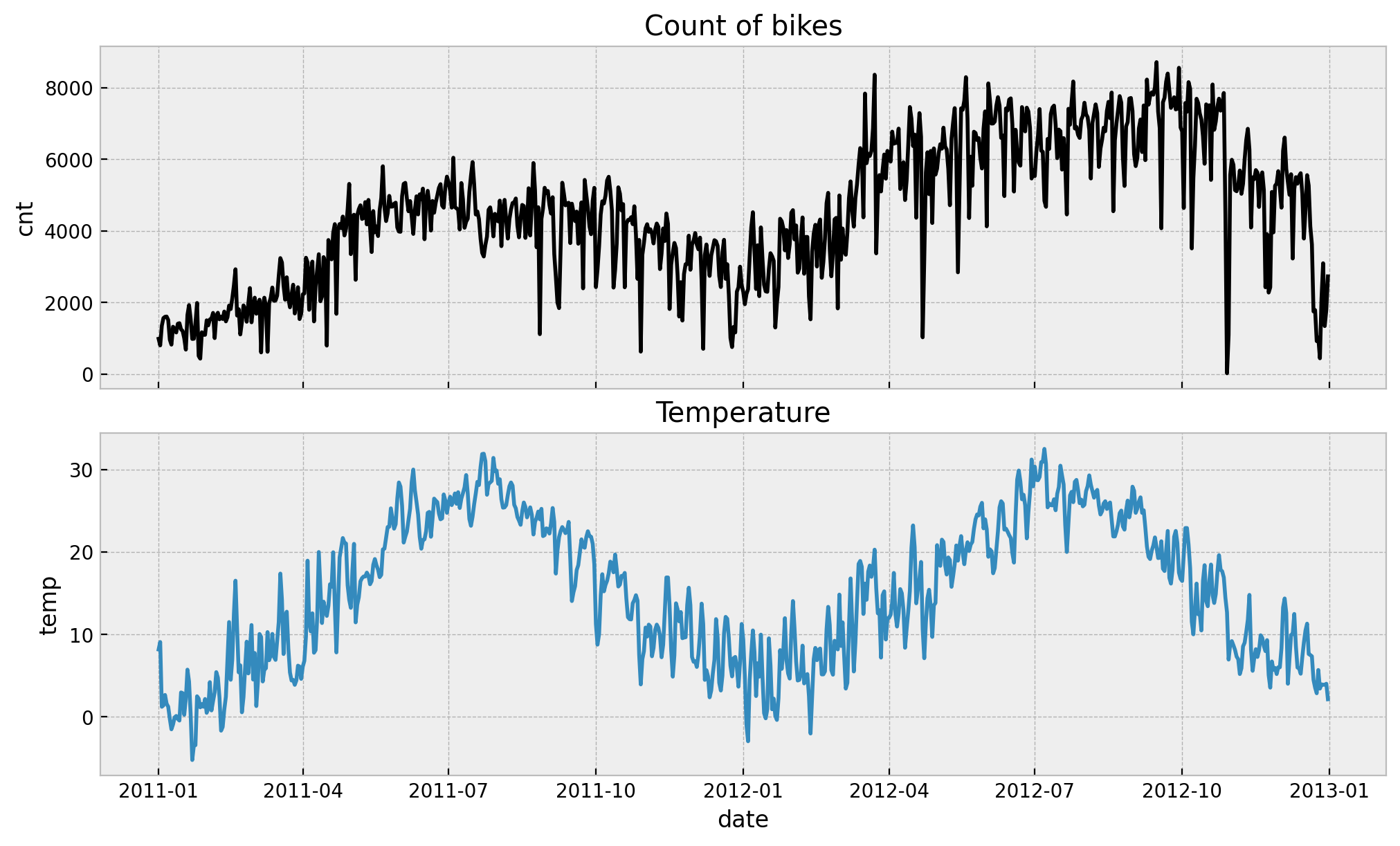
We add a Gaussian bump function to model the end-of-year seasonality.
is_december = data_df["date"].dt.month == 12
eoy_mu = 25
eoy_sigma = 7
eoy_arg = (data_df["date"].dt.day - eoy_mu) / eoy_sigma
data_df["eoy"] = is_december * np.exp(-(eoy_arg**2))

fig, ax = plt.subplots()
sns.lineplot(x="date", y="eoy", data=data_df, color="C4", ax=ax)
ax.set(title="End-of-Year Gaussian Bump")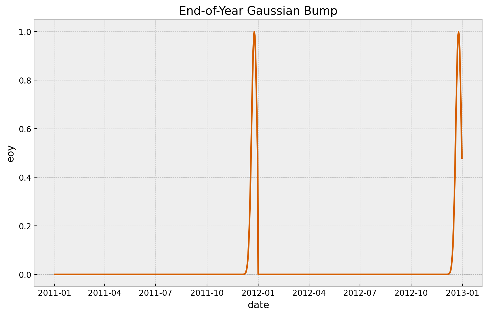
As we are going to fit a linear model is always good to scale the data.
target = "cnt"
target_scaled = f"{target}_scaled"

endog_scaler = MinMaxScaler()
exog_scaler = MinMaxScaler()


data_df[target_scaled] = endog_scaler.fit_transform(X=data_df[[target]])
data_df[["temp_scaled", "hum_scaled", "windspeed_scaled"]] = exog_scaler.fit_transform(
    X=data_df[["temp", "hum", "windspeed"]]
)
Finally, we extract the features we want to include in the model.
n = data_df.shape[0]
# target
cnt = data_df[target].to_numpy()
cnt_scaled = data_df[target_scaled].to_numpy()
# date feature
date = data_df["date"].to_numpy()
# model regressors
temp_scaled = data_df["temp_scaled"].to_numpy()
hum_scaled = data_df["hum_scaled"].to_numpy()
windspeed_scaled = data_df["windspeed_scaled"].to_numpy()
holiday_idx, holiday = data_df["holiday"].factorize(sort=True)
workingday_idx, workingday = data_df["workingday"].factorize(sort=True)
weathersit_idx, weathersit = data_df["weathersit"].factorize(sort=True)
t = data_df["days_since_2011"].to_numpy() / data_df["days_since_2011"].max()
eoy = data_df["eoy"].to_numpy()
Base Model
Before we jump into the time-varying coefficient model let us fist fit a baseline regression model. Let us follow the bayesian workflow for model development.
1. Model Specification
In a first step (after EDA and data pre-processing) we define the model structure. In particular we choose
- Prior distributions for the regression coefficients and the noise.
- Model parametrization, i.e. the structure of the linear model. Note that for the categorical variables we use a
ZeroSumNormalsince we are adding an intercept term. - Likelihood function, which is this case we decide for a StudentT distribution.
coords = {
    "date": date,
    "workingday": workingday,
    "weathersit": weathersit,
}

with pm.Model(coords=coords) as base_model:
    # --- priors ---
    intercept = pm.Normal(name="intercept", mu=0, sigma=2)
    b_temp = pm.Normal(name="b_temp", mu=0, sigma=1)
    b_hum = pm.Normal(name="b_hum", mu=0, sigma=1)
    b_windspeed = pm.Normal(name="b_windspeed", mu=0, sigma=1)
    b_holiday = pm.ZeroSumNormal(name="b_holiday", sigma=1, dims="holiday")
    b_workingday = pm.ZeroSumNormal(name="b_workingday", sigma=1, dims="workingday")
    b_weathersit = pm.ZeroSumNormal(name="b_weathersit", sigma=1, dims="weathersit")
    b_t = pm.Normal(name="b_t", mu=0, sigma=3)
    b_eoy = pm.Normal(name="b_eoy", mu=0, sigma=1)
    nu = pm.Gamma(name="nu", alpha=8, beta=2)
    sigma = pm.HalfNormal(name="sigma", sigma=1)

    # --- model parametrization ---
    mu = pm.Deterministic(
        name="mu",
        var=(
            intercept
            + b_t * t
            + b_temp * temp_scaled
            + b_hum * hum_scaled
            + b_windspeed * windspeed_scaled
            + b_holiday[holiday_idx]
            + b_workingday[workingday_idx]
            + b_weathersit[weathersit_idx]
            + b_eoy * eoy
        ),
        dims="date",
    )

    # --- likelihood ---
    likelihood = pm.StudentT(
        name="likelihood", mu=mu, nu=nu, sigma=sigma, dims="date", observed=cnt_scaled
    )


pm.model_to_graphviz(base_model)

2. Prior Predictive Analysis
We can analyze what the model expects before seeing the data.
with base_model:
    # --- prior samples ---
    prior_predictive_base = pm.sample_prior_predictive(samples=200, random_seed=rng)


palette = "viridis_r"
cmap = plt.get_cmap(palette)
percs = np.linspace(51, 99, 100)
colors = (percs - np.min(percs)) / (np.max(percs) - np.min(percs))


fig, ax = plt.subplots(figsize=(12, 6))

for i, p in enumerate(percs[::-1]):
    upper = np.percentile(
        prior_predictive_base.prior_predictive["likelihood"], p, axis=1
    )
    lower = np.percentile(
        prior_predictive_base.prior_predictive["likelihood"], 100 - p, axis=1
    )
    color_val = colors[i]
    ax.fill_between(
        x=date,
        y1=upper.flatten(),
        y2=lower.flatten(),
        color=cmap(color_val),
        alpha=0.1,
    )
sns.lineplot(x=date, y=cnt_scaled, color="black", ax=ax)
ax.set(
    title="Base Model - Prior Predictive Samples",
    xlabel="date",
    ylabel=target_scaled,
)
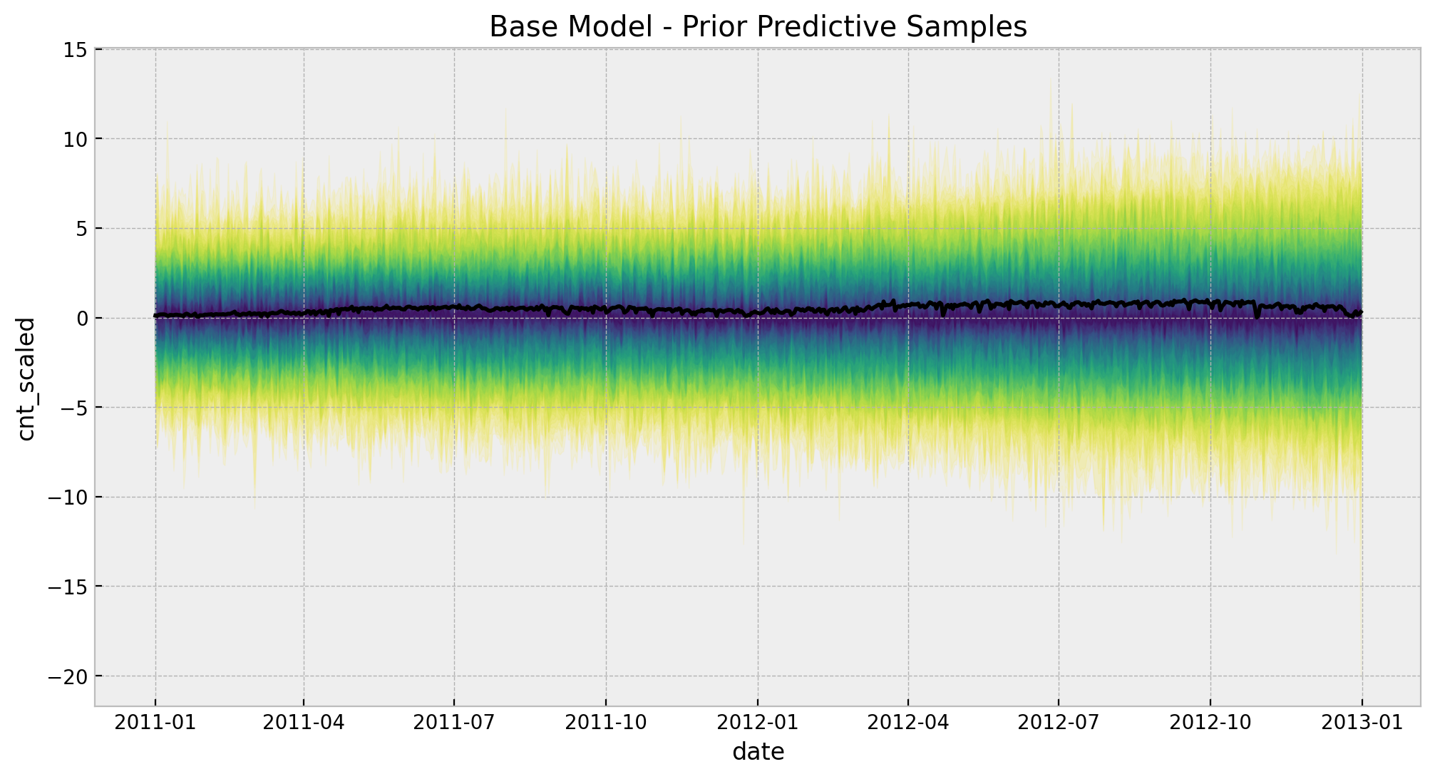
The chosen prior distributions are not very restrictive but they image of the predictions is still within a reasonable range.
3. Model Fit
We sample from the posterior distributions using the JAX based NUTS sampler from Numpyro.
with base_model:
    idata_base = pm.sample(
        target_accept=0.9,
        draws=2_000,
        chains=5,
        nuts_sampler="numpyro",
        idata_kwargs={"log_likelihood": True},
        random_seed=rng,
    )
    posterior_predictive_base = pm.sample_posterior_predictive(
        trace=idata, random_seed=rng
    )
# get number of divergences
idata_base["sample_stats"]["diverging"].sum().item()04. Model Diagnostics
Now wee look into some diagnostics metrics an plots.
az.summary(data=idata_base, var_names=["~mu"])
| mean | sd | hdi_3% | hdi_97% | mcse_mean | mcse_sd | ess_bulk | ess_tail | r_hat | |
|---|---|---|---|---|---|---|---|---|---|
| intercept | 0.096 | 0.031 | 0.039 | 0.155 | 0.000 | 0.000 | 4774.0 | 5867.0 | 1.0 |
| b_temp | 0.474 | 0.016 | 0.442 | 0.503 | 0.000 | 0.000 | 10817.0 | 7829.0 | 1.0 |
| b_hum | -0.155 | 0.032 | -0.216 | -0.096 | 0.000 | 0.000 | 6113.0 | 6706.0 | 1.0 |
| b_windspeed | -0.129 | 0.023 | -0.173 | -0.085 | 0.000 | 0.000 | 7584.0 | 6548.0 | 1.0 |
| b_t | 0.460 | 0.012 | 0.437 | 0.483 | 0.000 | 0.000 | 10465.0 | 7553.0 | 1.0 |
| b_eoy | -0.310 | 0.025 | -0.357 | -0.262 | 0.000 | 0.000 | 10741.0 | 7346.0 | 1.0 |
| b_holiday[HOLIDAY] | -0.025 | 0.011 | -0.045 | -0.005 | 0.000 | 0.000 | 9671.0 | 7367.0 | 1.0 |
| b_holiday[NO HOLIDAY] | 0.025 | 0.011 | 0.005 | 0.045 | 0.000 | 0.000 | 9671.0 | 7367.0 | 1.0 |
| b_workingday[NO WORKING DAY] | -0.007 | 0.004 | -0.014 | 0.000 | 0.000 | 0.000 | 12154.0 | 7185.0 | 1.0 |
| b_workingday[WORKING DAY] | 0.007 | 0.004 | -0.000 | 0.014 | 0.000 | 0.000 | 12154.0 | 7185.0 | 1.0 |
| b_weathersit[GOOD] | 0.086 | 0.009 | 0.068 | 0.103 | 0.000 | 0.000 | 5353.0 | 6721.0 | 1.0 |
| b_weathersit[MISTY] | 0.044 | 0.008 | 0.029 | 0.060 | 0.000 | 0.000 | 8161.0 | 7154.0 | 1.0 |
| b_weathersit[RAIN/SNOW/STORM] | -0.130 | 0.015 | -0.160 | -0.102 | 0.000 | 0.000 | 5753.0 | 6144.0 | 1.0 |
| nu | 4.816 | 0.812 | 3.363 | 6.345 | 0.009 | 0.006 | 8752.0 | 7263.0 | 1.0 |
| sigma | 0.077 | 0.003 | 0.070 | 0.084 | 0.000 | 0.000 | 8498.0 | 7483.0 | 1.0 |
axes = az.plot_trace(
    data=idata_base,
    var_names=["~mu"],
    compact=True,
    kind="rank_bars",
    backend_kwargs={"figsize": (12, 15), "layout": "constrained"},
)
plt.gcf().suptitle("Base Model - Trace", fontsize=16)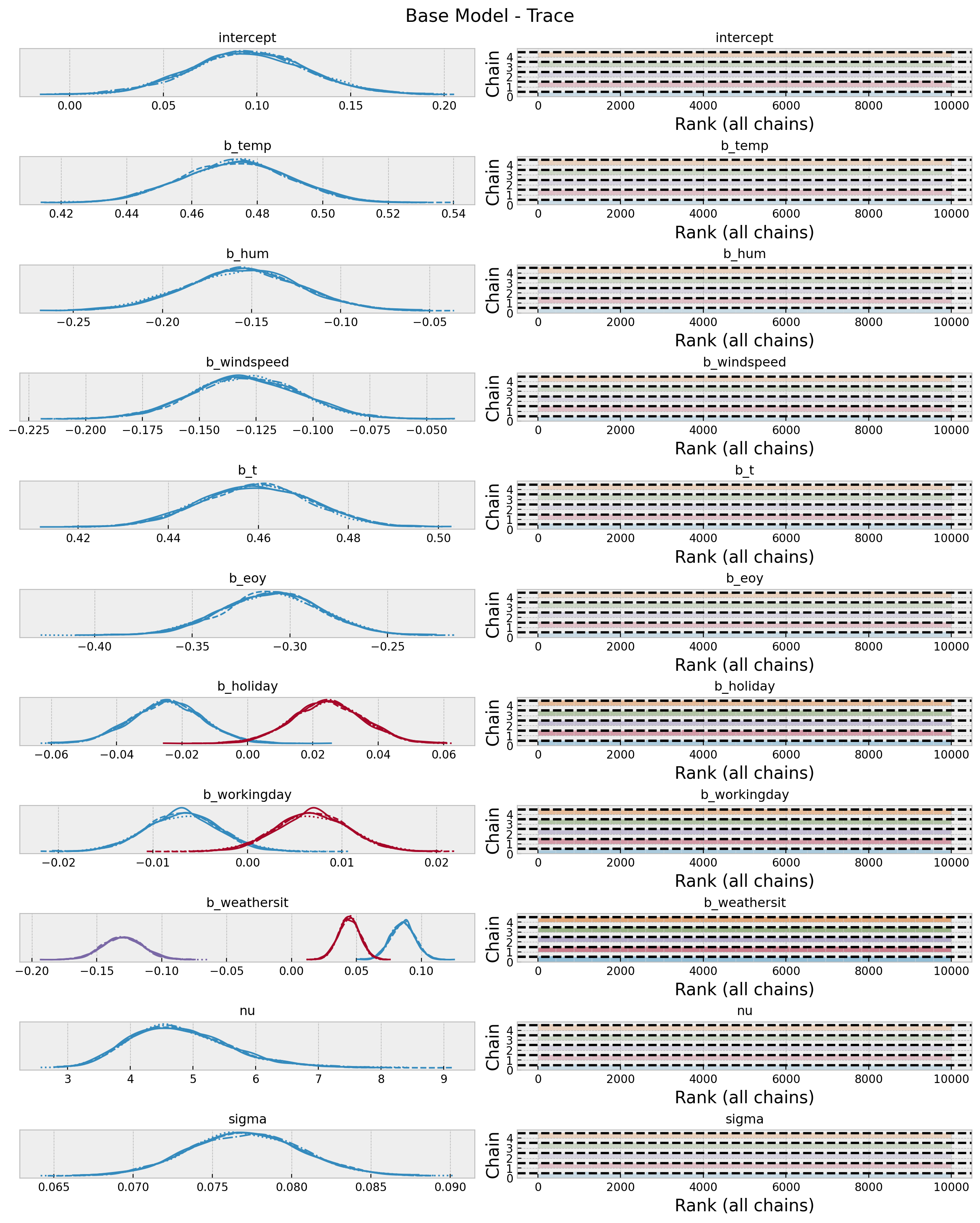
Overall, the model looks good.
axes = az.plot_forest(
    data=idata_base,
    var_names=["~mu", "~nu", "~sigma"],
    combined=True,
    r_hat=True,
    ess=True,
    figsize=(10, 6),
)
axes[0].axvline(x=0.0, color="black", linestyle="--")
plt.gcf().suptitle("Base Model - Posterior Distributions", fontsize=16)
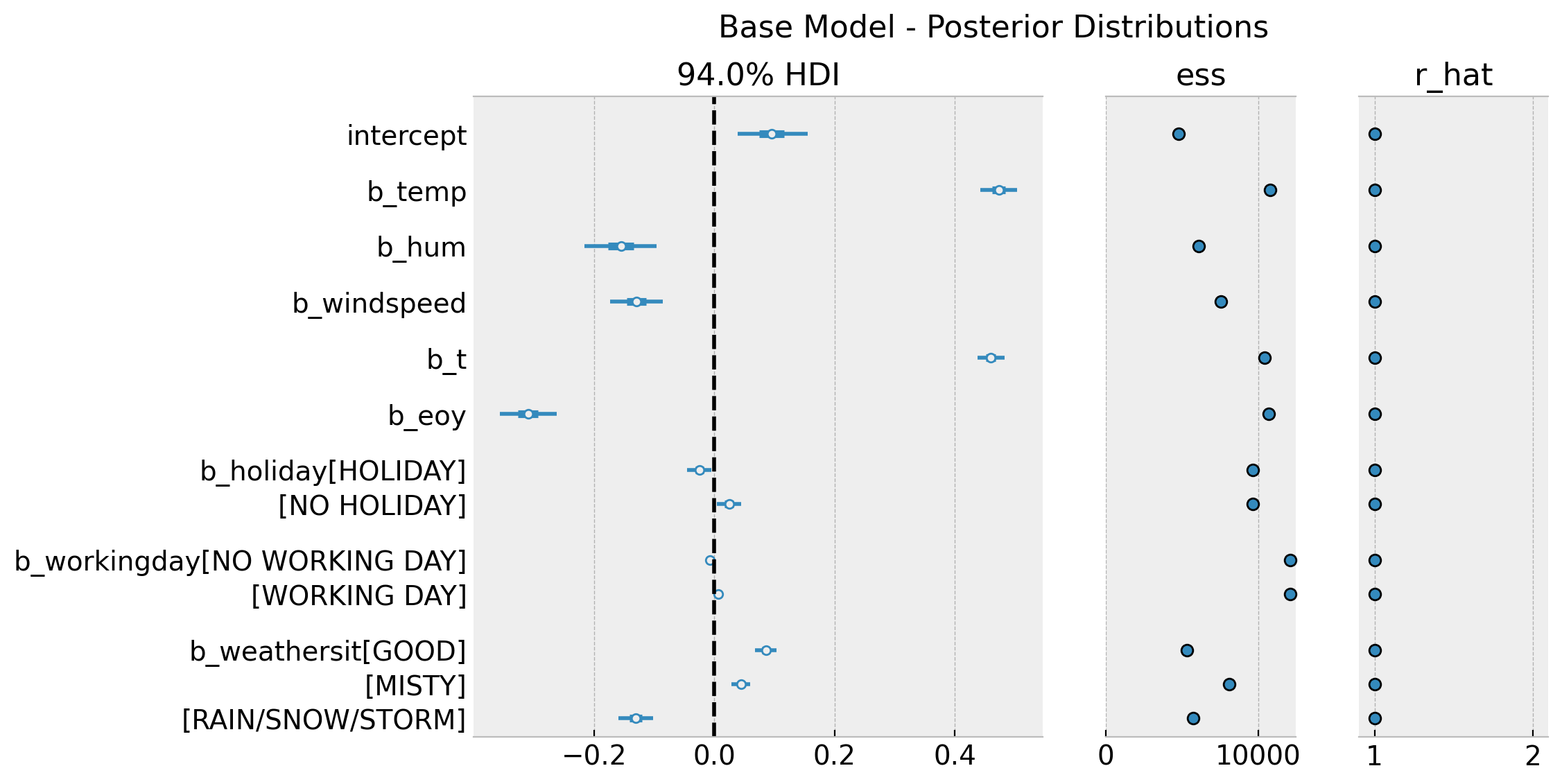
Note that in this base model the temperature feature has a positive effect on bike rentals on average.
5. Posterior Predictive Distribution
Finally, let us take a look at the fitted values.
palette = "viridis_r"
cmap = plt.get_cmap(palette)
percs = np.linspace(51, 99, 100)
colors = (percs - np.min(percs)) / (np.max(percs) - np.min(percs))


posterior_predictive_likelihood = posterior_predictive_base.posterior_predictive[
    "likelihood"
].stack(sample=("chain", "draw"))

posterior_predictive_likelihood_inv = endog_scaler.inverse_transform(
    X=posterior_predictive_likelihood.to_numpy()
)

fig, ax = plt.subplots(figsize=(12, 6))

for i, p in enumerate(percs[::-1]):
    upper = np.percentile(posterior_predictive_likelihood_inv, p, axis=1)
    lower = np.percentile(posterior_predictive_likelihood_inv, 100 - p, axis=1)
    color_val = colors[i]
    ax.fill_between(
        x=date,
        y1=upper,
        y2=lower,
        color=cmap(color_val),
        alpha=0.1,
    )

sns.lineplot(
    x=date,
    y=posterior_predictive_likelihood_inv.mean(axis=1),
    color="C2",
    label="posterior predictive mean",
    ax=ax,
)
sns.lineplot(
    x=date,
    y=cnt,
    color="black",
    label=target,
    ax=ax,
)
ax.legend(loc="upper left")
ax.set(
    title="Base Model - Posterior Predictive Samples",
    xlabel="date",
    ylabel=target,
)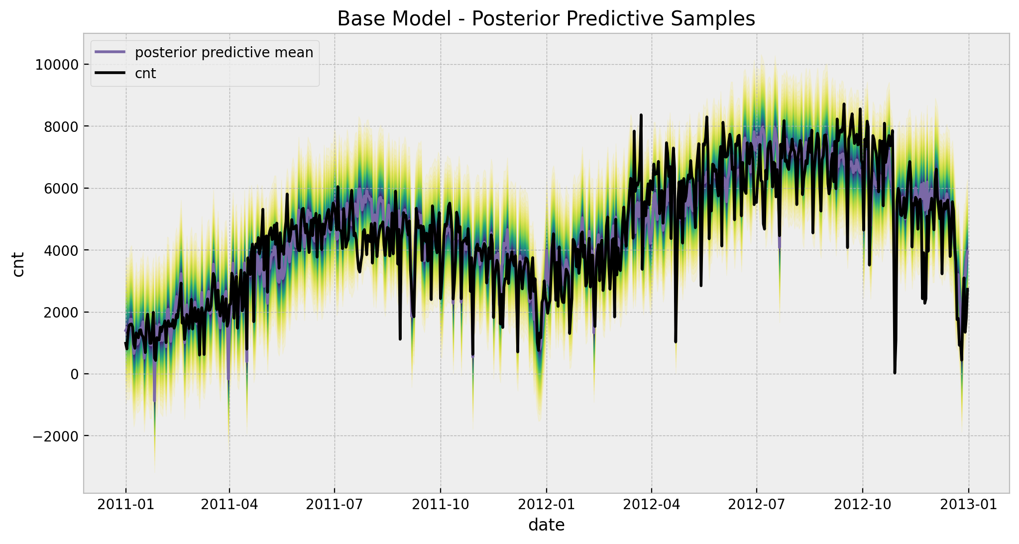
Observe that for certain points in July the predictions and the fit do not coincide and go in opposite directions. This will be solved by adding the time-varying coefficient to the linear model for the temperature regressor (see below).
Remark: Note that the model predict negative values for the bike rentals. This is of course not good! An alterative choice of likelihood to model count data would resolve this (e.g. Poisson or Negative Binomial likelihoods).
Time-Varying Coefficients Model
We now follow the same workflow above. The main difference is that we replace the regression coefficient of the temperature with GaussianRandomWalk and remove the intercept term.
1. Model Specification
with pm.Model(coords=coords) as model:
    # --- priors ---
    b_hum = pm.Normal(name="b_hum", mu=0, sigma=1)
    b_windspeed = pm.Normal(name="b_windspeed", mu=0, sigma=1)
    b_holiday = pm.ZeroSumNormal(name="b_holiday", sigma=1, dims="holiday")
    b_workingday = pm.ZeroSumNormal(name="b_workingday", sigma=1, dims="workingday")
    b_weathersit = pm.ZeroSumNormal(name="b_weathersit", sigma=1, dims="weathersit")
    b_t = pm.Normal(name="b_t", mu=0, sigma=2)
    b_eoy = pm.Normal(name="b_eoy", mu=0, sigma=1)
    sigma_slopes = pm.Exponential(name="sigma_slope", lam=1 / 0.2)
    nu = pm.Gamma(name="nu", alpha=8, beta=2)
    sigma = pm.HalfNormal(name="sigma", sigma=1)

    # --- model parametrization ---
    slopes = pm.GaussianRandomWalk(
        name="slopes",
        sigma=sigma_slopes,
        init_dist=Exponential.dist(lam=1 / 0.1),
        dims="date",
    )
    mu = pm.Deterministic(
        name="mu",
        var=(
            b_t * t
            + slopes * temp_scaled
            + b_hum * hum_scaled
            + b_windspeed * windspeed_scaled
            + b_holiday[holiday_idx]
            + b_workingday[workingday_idx]
            + b_weathersit[weathersit_idx]
            + b_eoy * eoy
        ),
        dims="date",
    )

    # --- likelihood ---
    likelihood = pm.StudentT(
        name="likelihood", mu=mu, nu=nu, sigma=sigma, dims="date", observed=cnt_scaled
    )


pm.model_to_graphviz(model)
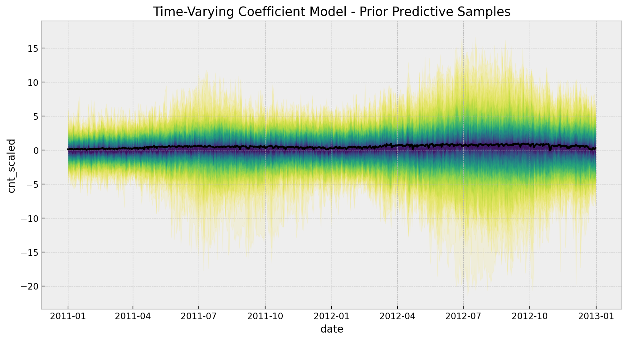
2. Prior Predictive Analysis
with model:
    # --- prior samples ---
    prior_predictive = pm.sample_prior_predictive(samples=200, random_seed=rng)


palette = "viridis_r"
cmap = plt.get_cmap(palette)
percs = np.linspace(51, 99, 100)
colors = (percs - np.min(percs)) / (np.max(percs) - np.min(percs))


fig, ax = plt.subplots(figsize=(12, 6))

for i, p in enumerate(percs[::-1]):
    upper = np.percentile(prior_predictive.prior_predictive["likelihood"], p, axis=1)
    lower = np.percentile(
        prior_predictive.prior_predictive["likelihood"], 100 - p, axis=1
    )
    color_val = colors[i]
    ax.fill_between(
        x=date,
        y1=upper.flatten(),
        y2=lower.flatten(),
        color=cmap(color_val),
        alpha=0.1,
    )
sns.lineplot(x=date, y=cnt_scaled, color="black", ax=ax)
ax.set(
    title="Time-Varying Coefficient Model - Prior Predictive Samples",
    xlabel="date",
    ylabel=target_scaled,
)
3. Model Fit
with model:
    idata = pm.sample(
        target_accept=0.97,
        draws=2_000,
        chains=5,
        nuts_sampler="numpyro",
        idata_kwargs={"log_likelihood": True},
        random_seed=rng,
    )
    posterior_predictive = pm.sample_posterior_predictive(
        trace=idata, random_seed=rng
    )
# get number of divergences
idata["sample_stats"]["diverging"].sum().item()
13We get a small number of divergences 😔 … still not dramatic.
4. Model Diagnostics
az.summary(data=idata, var_names=["~mu", "~slopes"])| mean | sd | hdi_3% | hdi_97% | mcse_mean | mcse_sd | ess_bulk | ess_tail | r_hat | |
|---|---|---|---|---|---|---|---|---|---|
| b_hum | -0.077 | 0.019 | -0.112 | -0.040 | 0.001 | 0.001 | 656.0 | 2021.0 | 1.00 |
| b_windspeed | -0.082 | 0.016 | -0.111 | -0.052 | 0.000 | 0.000 | 2182.0 | 5512.0 | 1.00 |
| b_t | 0.399 | 0.033 | 0.336 | 0.459 | 0.004 | 0.003 | 87.0 | 424.0 | 1.06 |
| b_eoy | -0.248 | 0.037 | -0.316 | -0.175 | 0.001 | 0.001 | 1852.0 | 3498.0 | 1.00 |
| b_holiday[HOLIDAY] | -0.043 | 0.008 | -0.057 | -0.027 | 0.000 | 0.000 | 2628.0 | 6585.0 | 1.00 |
| b_holiday[NO HOLIDAY] | 0.043 | 0.008 | 0.027 | 0.057 | 0.000 | 0.000 | 2628.0 | 6585.0 | 1.00 |
| b_workingday[NO WORKING DAY] | -0.005 | 0.003 | -0.010 | -0.000 | 0.000 | 0.000 | 12229.0 | 9441.0 | 1.00 |
| b_workingday[WORKING DAY] | 0.005 | 0.003 | 0.000 | 0.010 | 0.000 | 0.000 | 12229.0 | 9441.0 | 1.00 |
| b_weathersit[GOOD] | 0.102 | 0.006 | 0.090 | 0.113 | 0.000 | 0.000 | 2059.0 | 5124.0 | 1.00 |
| b_weathersit[MISTY] | 0.049 | 0.007 | 0.037 | 0.062 | 0.000 | 0.000 | 5743.0 | 7402.0 | 1.00 |
| b_weathersit[RAIN/SNOW/STORM] | -0.151 | 0.011 | -0.172 | -0.129 | 0.000 | 0.000 | 2845.0 | 5447.0 | 1.00 |
| sigma_slope | 0.044 | 0.006 | 0.033 | 0.055 | 0.000 | 0.000 | 212.0 | 347.0 | 1.02 |
| nu | 2.564 | 0.349 | 1.925 | 3.204 | 0.006 | 0.004 | 3667.0 | 7415.0 | 1.00 |
| sigma | 0.042 | 0.003 | 0.035 | 0.048 | 0.000 | 0.000 | 811.0 | 2206.0 | 1.01 |
axes = az.plot_trace(
    data=idata,
    var_names=["~mu", "~slopes"],
    compact=True,
    kind="rank_bars",
    backend_kwargs={"figsize": (12, 15), "layout": "constrained"},
)
plt.gcf().suptitle("Time-Varying Coefficient Model - Trace", fontsize=16)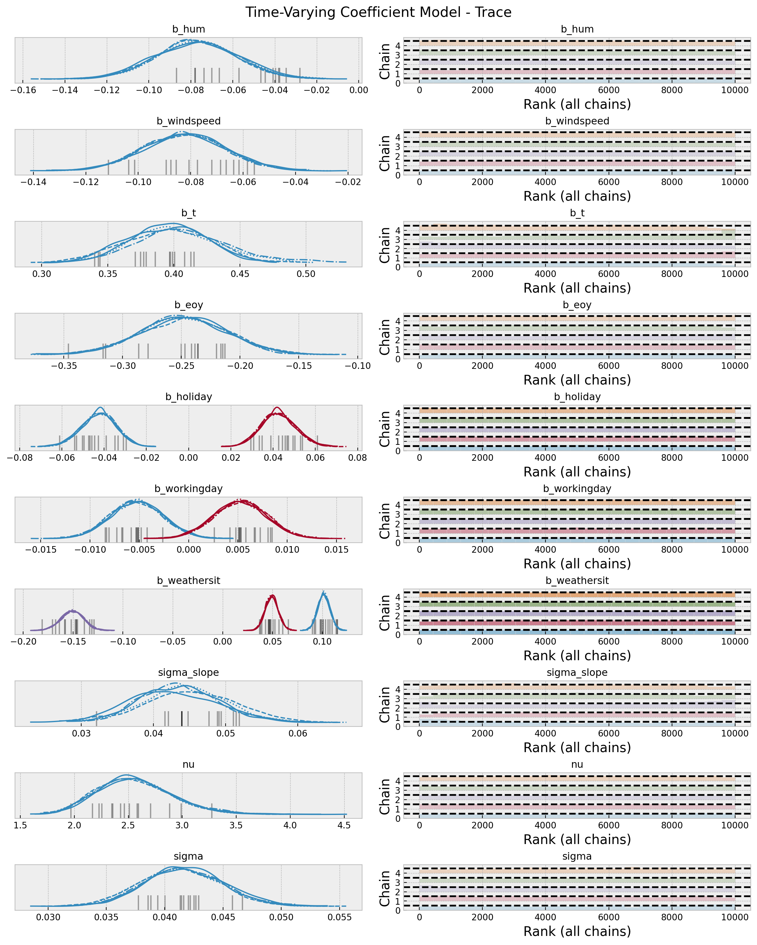
Let us now compare the two models in a forest plot.
axes = az.plot_forest(
    data=[idata_base, idata],
    model_names=["base", "time-varying"],
    var_names=["~mu", "~slopes", "~nu", "~sigma"],
    combined=True,
    r_hat=True,
    ess=True,
    figsize=(12, 7),
)
axes[0].axvline(x=0.0, color="black", linestyle="--")
plt.gcf().suptitle("Posterior Distributions", fontsize=16)
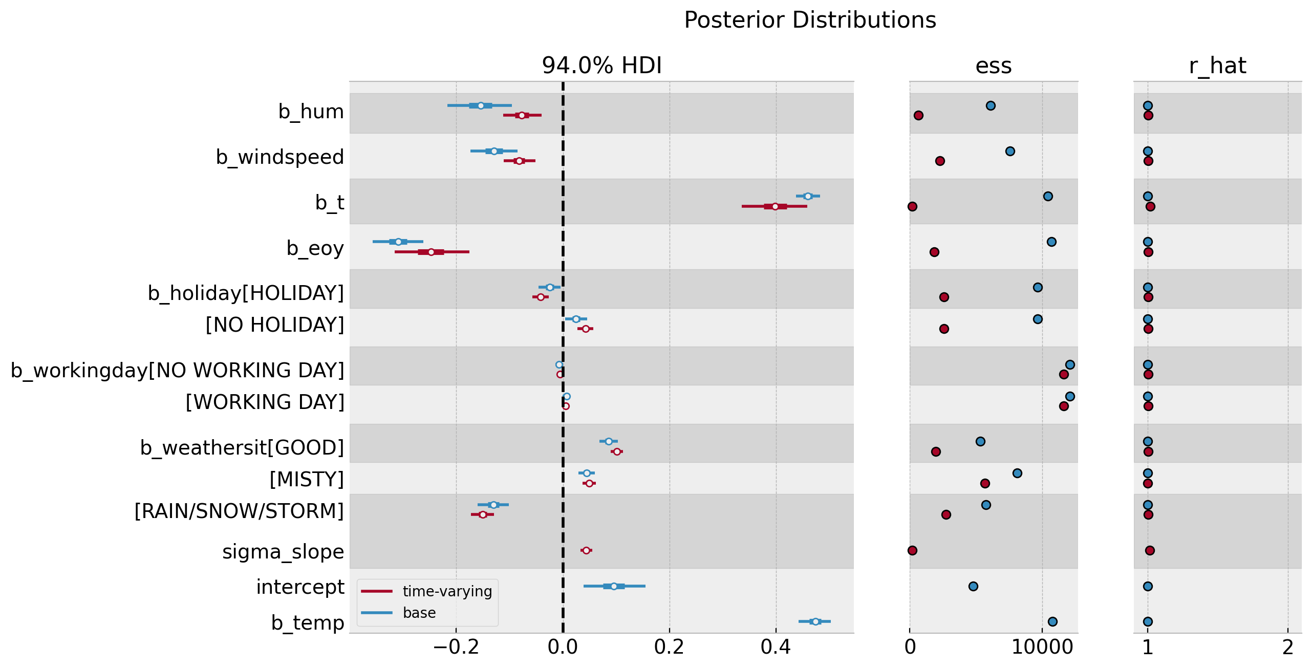
Overall, there is no major change in the estimated regression coefficients besides the trend component.
We can also use the az.compare method to compare the two models.
az.compare(compare_dict={"base": idata_base, "time-varying": idata})
| rank | elpd_loo | p_loo | elpd_diff | weight | se | dse | warning | scale | |
|---|---|---|---|---|---|---|---|---|---|
| time-varying | 0 | 859.510979 | 190.554494 | 0.000000 | 0.924529 | 28.507826 | 0.000000 | False | log |
| base | 1 | 668.611994 | 11.713275 | 190.898985 | 0.075471 | 24.952297 | 21.054906 | False | log |
It seems that the time-varying coefficient model is better at predicting the bike rentals.
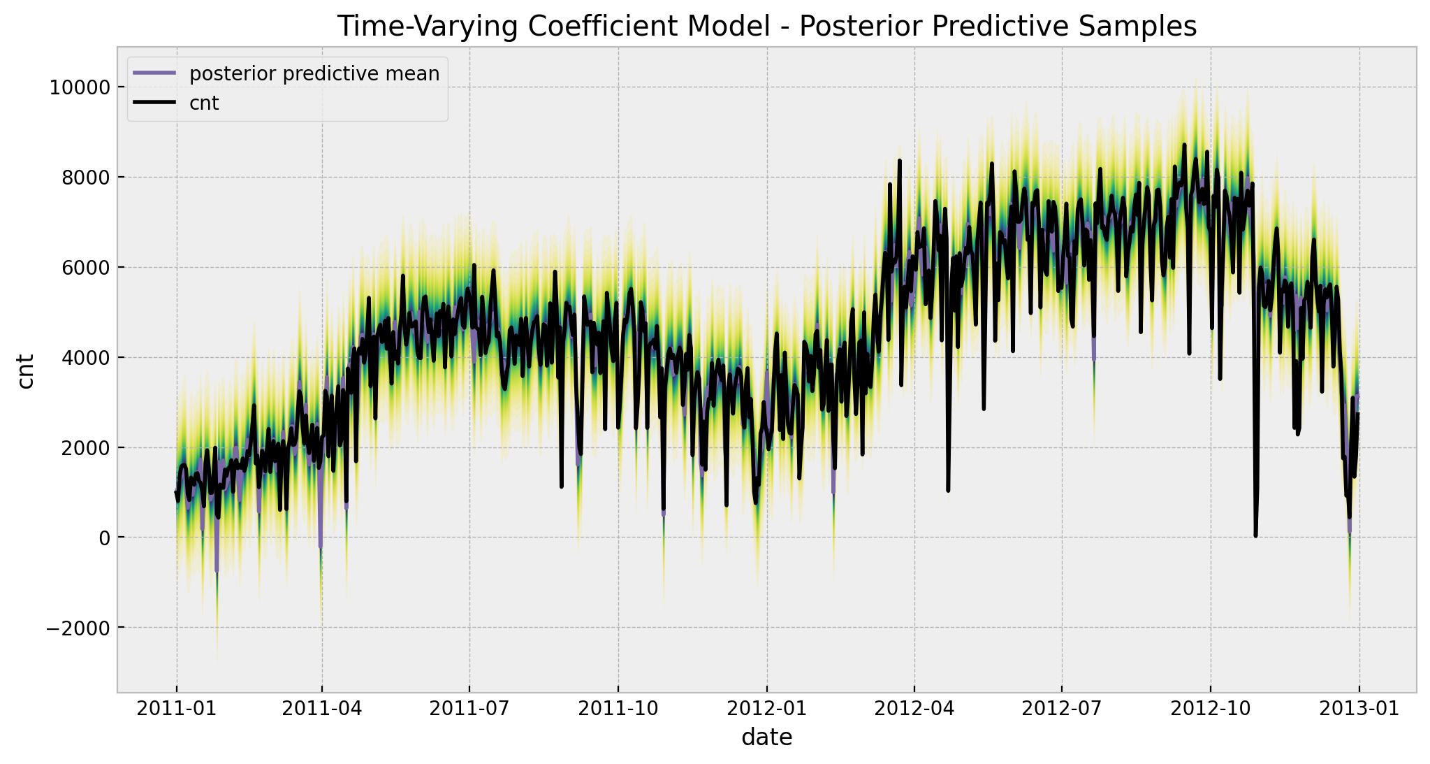
5. Posterior Predictive Distribution
palette = "viridis_r"
cmap = plt.get_cmap(palette)
percs = np.linspace(51, 99, 100)
colors = (percs - np.min(percs)) / (np.max(percs) - np.min(percs))


posterior_predictive_likelihood = posterior_predictive.posterior_predictive[
    "likelihood"
].stack(sample=("chain", "draw"))

posterior_predictive_likelihood_inv = endog_scaler.inverse_transform(
    X=posterior_predictive_likelihood.to_numpy()
)

fig, ax = plt.subplots(figsize=(12, 6))

for i, p in enumerate(percs[::-1]):
    upper = np.percentile(posterior_predictive_likelihood_inv, p, axis=1)
    lower = np.percentile(posterior_predictive_likelihood_inv, 100 - p, axis=1)
    color_val = colors[i]
    ax.fill_between(
        x=date,
        y1=upper,
        y2=lower,
        color=cmap(color_val),
        alpha=0.1,
    )

sns.lineplot(
    x=date,
    y=posterior_predictive_likelihood_inv.mean(axis=1),
    color="C2",
    label="posterior predictive mean",
    ax=ax,
)
sns.lineplot(
    x=date,
    y=cnt,
    color="black",
    label=target,
    ax=ax,
)
ax.legend(loc="upper left")
ax.set(
    title="Time-Varying Coefficient Model - Posterior Predictive Samples",
    xlabel="date",
    ylabel=target,
)
6. Temperature Effect Deep-Dive
Next, we wan to compare the inferred temperature effect from both models. To begin with, let us compare the mean effect for both models.
base_tmp_mean = (
    idata_base.posterior["b_temp"].stack(sample=("chain", "draw")).to_numpy().mean()
)
time_varying_tmp_mean = (
    idata.posterior["slopes"].stack(sample=("chain", "draw")).to_numpy().mean()
)
print(
    f"""
base model mean effect = {base_tmp_mean: 0.3f}
------------------------------------------
time-varying model mean effect  = {time_varying_tmp_mean: 0.3f}
------------------------------------------
"""
)
base model mean effect = 0.473
------------------------------------------
time-varying model mean effect = 0.536
------------------------------------------It seems that the effect of the time-varying coefficient model is higher. Still, this is just one statistic.It is always better to see the data. The following plot shows the effect as a function of the temperature.
fig, ax = plt.subplots(figsize=(12, 7))
sns.scatterplot(
    x="temp",
    y="slopes",
    data=data_df.assign(slopes=idata.posterior["slopes"].mean(dim=["chain", "draw"])),
    hue="mnth",
    palette="tab20",
)
sns.lineplot(
    x="temp",
    y="b_temp",
    data=data_df.assign(
        b_temp=idata_base.posterior["b_temp"].mean(dim=["chain", "draw"]).to_numpy()
    ),
    color="black",
    label="base model",
    ax=ax,
)
sns.rugplot(x=data_df["temp"], color="black", alpha=0.5, ax=ax)
ax.axhline(y=0.0, color="gray", linestyle="--")
ax.legend(loc="center left", bbox_to_anchor=(1, 0.5))
ax.set(title="Temperature Effect", xlabel="temp", ylabel="effect")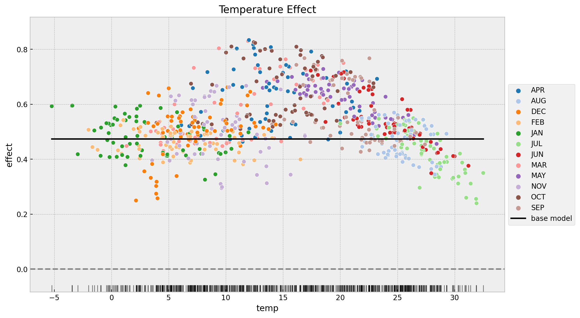
We see many interesting features from this plot:
- The time-varying coefficient model indeed finds a non constant effect of temperature on bike rentals.
- The effect of second model is always positive and starts decreasing at around \(15\) degrees which is consistent with the results found in the previous post Exploring Tools for Interpretable Machine Learning.
- The lowest points of the effect are:
- December and January. I think this is some seasonality effect that is not captured by the model.
- During the summer months when the temperatures are very high, the effect decreases considerably.
- The variance of the time-varying effect decreases with the temperature.
Next, we plot the temperature effect as a function of time.
palette = "cividis_r"
cmap = plt.get_cmap(palette)
percs = np.linspace(51, 99, 100)
colors = (percs - np.min(percs)) / (np.max(percs) - np.min(percs))


posterior_predictive_slopes = idata.posterior["slopes"].stack(sample=("chain", "draw"))

fig, ax = plt.subplots(
    nrows=2, ncols=1, figsize=(10, 6), sharex=True, sharey=False, layout="constrained"
)

for i, p in enumerate(percs[::-1]):
    upper = np.percentile(posterior_predictive_slopes, p, axis=1)
    lower = np.percentile(posterior_predictive_slopes, 100 - p, axis=1)
    color_val = colors[i]
    ax[0].fill_between(
        x=date,
        y1=upper,
        y2=lower,
        color=cmap(color_val),
        alpha=0.1,
    )

sns.lineplot(
    x="date",
    y="b_temp",
    data=data_df.assign(
        b_temp=idata_base.posterior["b_temp"]
        .stack(sample=("chain", "draw"))
        .mean()
        .to_numpy()
    ),
    color="black",
    label="base model",
    ax=ax[0],
)
ax[0].axhline(y=0.0, color="gray", linestyle="--")
ax[0].legend(loc="upper left")
ax[0].set(title="Temperature Effect")
sns.lineplot(x="date", y="temp", data=data_df, color="C0", ax=ax[1])
ax[1].set(title="Temperature")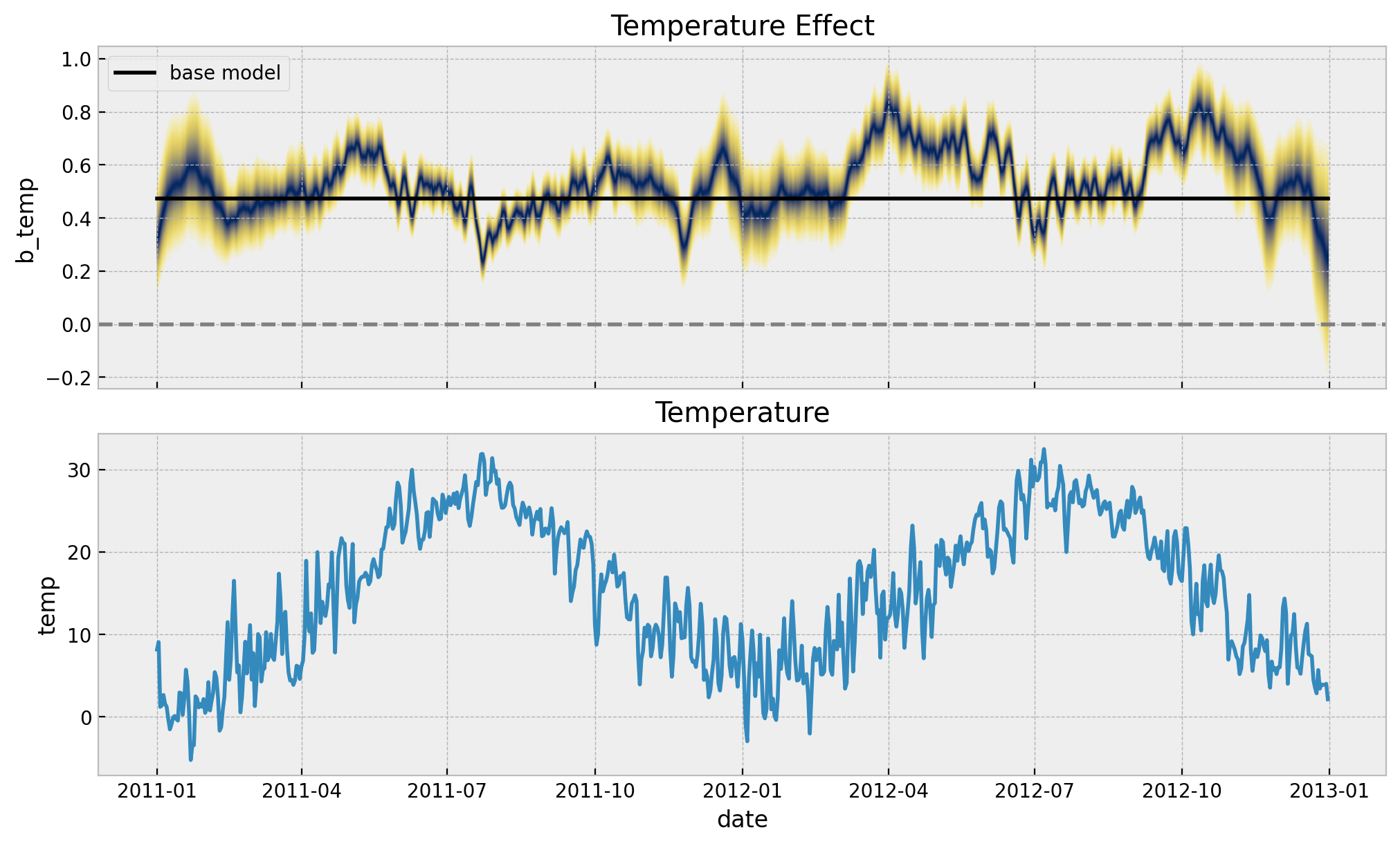
In the time-varying coefficient model, the temperature effect oscillates around the constant effect of the baseline model. We do see that during the spring months the effect is higher than the constant effect of the baseline model. This is consistent with the previous plot.
We can transform the scale back into the original scale:
temp_effect_scaled_baseline = (
    idata_base["posterior"]["b_temp"] * exog_scaler.scale_[0]
) / endog_scaler.scale_[0]

temp_effect_scaled = (
    idata["posterior"]["slopes"] * exog_scaler.scale_[0]
) / endog_scaler.scale_[0]

fig, ax = plt.subplots(figsize=(12, 7))
az.plot_hdi(
    x=data_df["temp"].to_numpy(),
    y=temp_effect_scaled,
    hdi_prob=0.94,
    color="C0",
    fill_kwargs={"alpha": 0.4, "label": "$94\%$ HDI"},
    ax=ax,
)
az.plot_hdi(
    x=data_df["temp"].to_numpy(),
    y=temp_effect_scaled,
    hdi_prob=0.5,
    color="C0",
    fill_kwargs={"alpha": 0.6, "label": "$50\%$ HDI"},
    ax=ax,
)
ax.axhline(
    y=temp_effect_scaled_baseline.mean(dim=["chain", "draw"]).item(),
    color="C1",
    linestyle="--",
    label="base model posterior predictive mean",
)
sns.rugplot(x=data_df["temp"], color="black", alpha=0.5, ax=ax)
ax.axhline(y=0.0, color="gray", linestyle="--")
ax.legend(loc="upper right")
ax.set(
    title="Temperature Coefficient (Original Scale) - Posterior Predictive",
    xlabel="temp",
    ylabel=None,
)
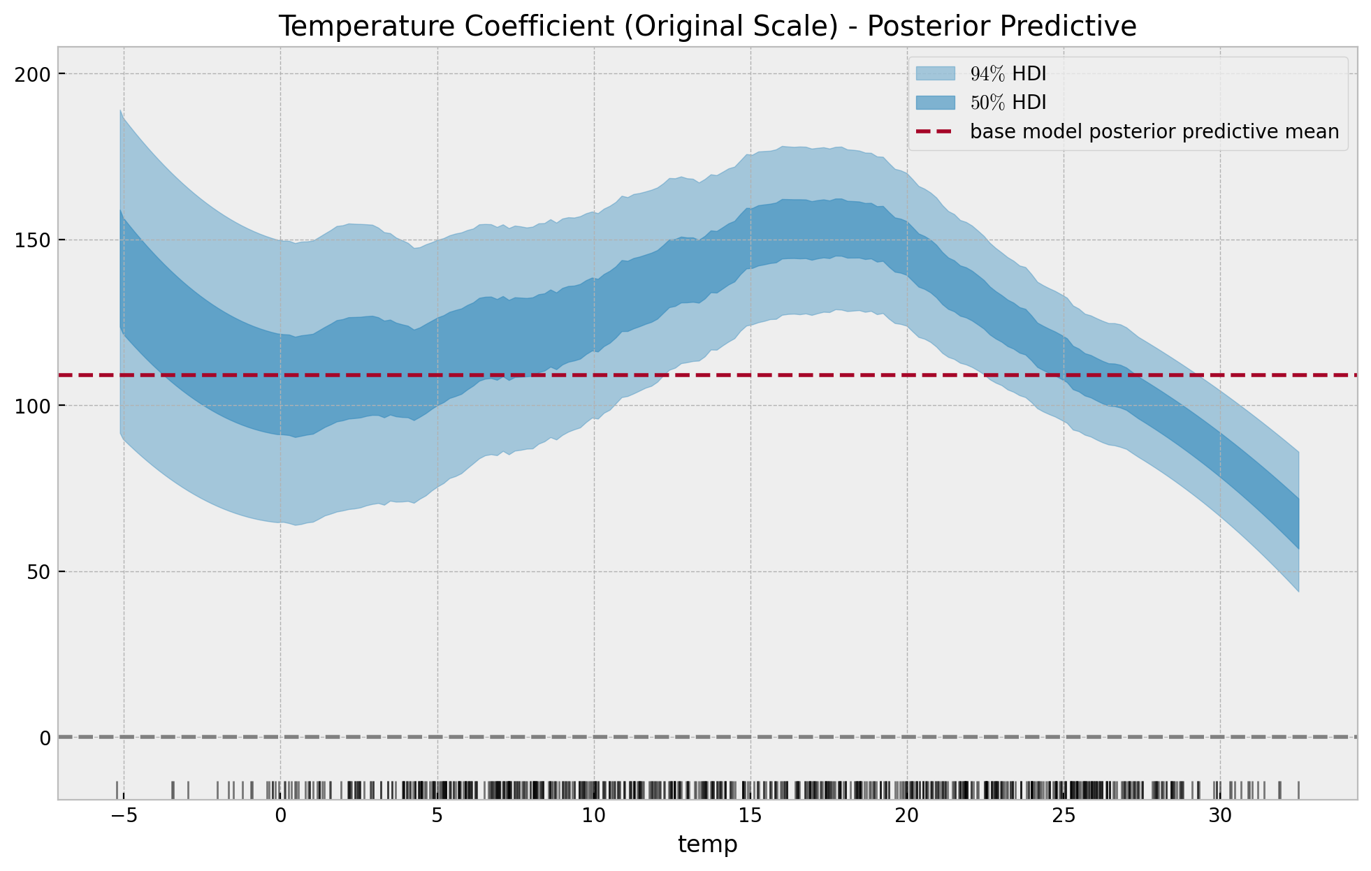
For temperatures lower than \(-2\) the estimate is noisy and is probably leaking some seasonality effects.
Note that these results are compatible with the insights found on the previous post Exploring Tools for Interpretable Machine Learning. For example, take a look into the PDP and ICE Pots

and specifically here is are the same plots restricted to the month of July:

Here we see the negative effect of temperature on bike count for the summer months.
Remark: It would be interesting to compare these results with Orbit’s KTR model (see Media Effect Estimation with Orbit’s KTR Model)