Motivated by the nice talk on Winning with Simple, even Linear, Models by Vincent D. Warmerdam, I briefly describe how to construct certain class of bump functions to encode seasonal variables in R.
Prepare Notebook
library(glue)
library(lubridate)
library(magrittr)
library(tidyverse)
Generate Data
Let us generate a time sequence variable stored in a tibble.
# Define time sequence.
t <- seq.Date(from = as.Date("2017-07-01"), to = as.Date("2019-04-01"), by = "day")
# Store it in a tibble.
df <- tibble(t = t)
Symmetric Bump Function
We want to generate a gaussian-like curve around a specific date. The width of the bump function is parametrized by a non-negative number \(\varepsilon \geq 0\). For \(\varepsilon = 0\) we generate a dummy variable. Namely, for \(\varepsilon \neq 0\),
\[ f_{x_0, \varepsilon}(x) = \exp\left(- \left(\frac{x - x_0}{\varepsilon}\right)^2 \right) \]
In R,
bump_func <- function(x, x_0 = 0, epsilon = 1) {
  # If `epsilon` = 0, we encode it as a dummy variable.
  if (epsilon == 0) {
    as.numeric(x == x_0)
  } else {
    delta <-  as.numeric(x - x_0)
    exp(- (delta / epsilon)^2)
  }
}
Examples
Let us asumme we want to model the effect of Christmas 2018-12-24.
- \(\varepsilon = 0\) will generate a dummy variable.
epsilon <- 0

df %>%
  mutate(y = bump_func(x = t,
                       x_0 = as.Date("2018-12-24"),
                       epsilon = epsilon)) %>%
  ggplot() +
  geom_line(mapping = aes(x = t, y = y)) +
  xlab("Date") +
  ylab("") +
  ggtitle(label = glue("Bump Seasonal Variable - epsilon = {epsilon}"))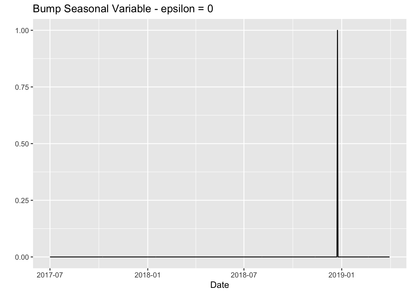
- \(\varepsilon = 8\) will generate a bump function around
2018-12-24.
epsilon <- 8

df %>%
  mutate(y = bump_func(x = t,
                       x_0 = as.Date("2018-12-24"),
                       epsilon = 8)) %>%
  ggplot() +
  geom_line(mapping = aes(x = t, y = y)) +
  xlab("Date") +
  ylab("") +
  ggtitle(label = glue("Bump Seasonal Variable - epsilon = {epsilon}"))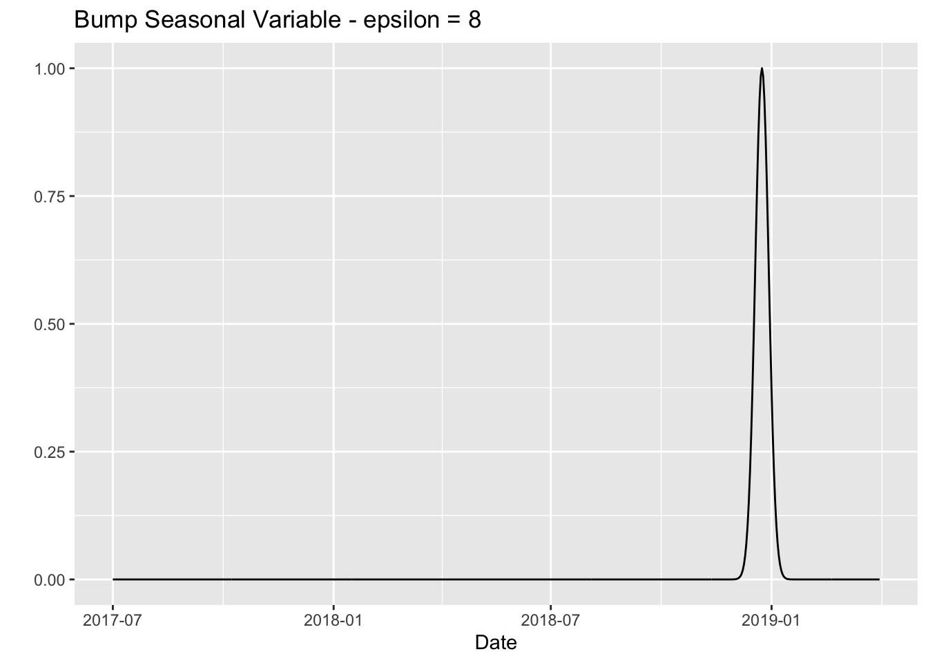
Let us see how to do it for repeated dates and events:
epsilon <- 8

christmas_dates <- c(as.Date("2017-12-24"), as.Date("2018-12-24"))
halloween_dates <- c(as.Date("2017-10-31"), as.Date("2018-10-31"))

df %>%
  mutate(
    y_christmas = map(
      .x = christmas_dates,
      .f = ~ bump_func(x = t, x_0 = .x, epsilon = epsilon)) %>%
      reduce(.f = ~ .x + .y),

    y_halloween = map(
      .x = halloween_dates,
      .f = ~ bump_func(x = t, x_0 = .x, epsilon = epsilon)) %>%
      reduce(.f = ~ .x + .y)) %>%
  gather(key = Event, value = value, ... = y_christmas, y_halloween) %>%
  # Plot variables.
  ggplot() +
  geom_line(mapping = aes(x = t, y = value, color = Event)) +
  xlab("Date") +
  ylab("") +
  ggtitle(label = glue("Bump Seasonal Variable - epsilon = {epsilon}"))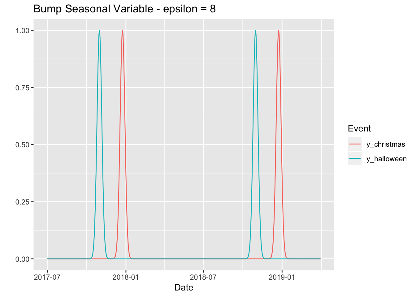
Asymmetric Bump Function
Sometimes the effect before and after the seasonal variable is note the same. To model this we can tweak the bump function defined above so that:
- It is not symmetric.
- It can have a drop after the seasonal variable (an potentially have different effect sizes).
A natural candidate to fulfill these requirements is
\[ a_{-} f_{x_0, \varepsilon_{-}}(x)I_{\{x \leq x_0\}} \pm a_{+} f_{x_0, \varepsilon_{+}}(x) I_{\{x > x_0\}} \] where:
\(I_{\{x \leq x_0\}}\) and \(I_{\{x > x_0\}}\) denote the corresponing indicator functions.
\(f_{x_0, \varepsilon_{\pm}}\) denotes the bump function defined above.
\(\varepsilon_{-}, \varepsilon_{+} >0\) denote the width (variance) before and after \(x_0\) respectively.
\(a_{-}, a_{+} >0\) denote the amplitudes before and after \(x_0\) respectively.
We now write this function in R.
asymmestric_bump_func <- function(
  # Input vector.
  x,
  # Maximum of bump function.
  x_0,
  # Width of bump function before `x_0`.
  epsilon_minus = 1,
  # Width of bump function after `x_0`.
  epsilon_plus = 1,
  # Amplitude of bump function before `x_0`.
  a_minus = 1,
  # Amplitude of bump function after `x_0`.
  a_plus = 1,
  # Wether to have a drom after `x_0`.
  drop = FALSE
  ) {

  delta <- as.numeric(x - x_0)
  # Define indicator functions.
  indicator_minus <- as.numeric(delta < 0)
  indicator_plus <- as.numeric(delta >= 0)

  # Calculate bump function components.
  y_minus <- a_minus * indicator_minus * bump_func(x = x, x_0 = x_0, epsilon = epsilon_minus)
  y_plus <- a_plus*indicator_plus * bump_func(x = x, x_0 = x_0, epsilon = epsilon_plus)
  # Calculate sign depending on the drop choice.
  drop_sign <- 2*as.numeric(drop) - 1

  y <- y_minus  - drop_sign*y_plus

  return(y)
}
Examples
Let us ilustrate the results for Christmas 2017-12-24.
Without Drop
df  %>%
  mutate(y =  asymmestric_bump_func(x = t,
                                    x_0 = as.Date("2017-12-24"),
                                    epsilon_minus = 20,
                                    epsilon_plus = 4,
                                    drop = FALSE)) %>%
  # Filter for visualization (zoom in).
  filter(t < "2018-02-01") %>%
  ggplot() +
  geom_line(mapping = aes(x = t, y = y)) +
  xlab("Date") +
  ylab("") +
  ggtitle(label = glue("Asymmetric Bump Function"))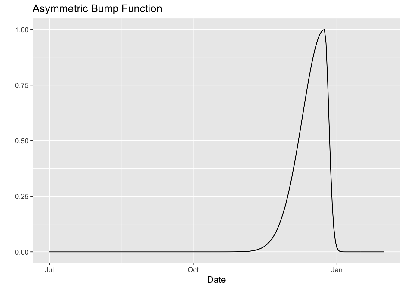
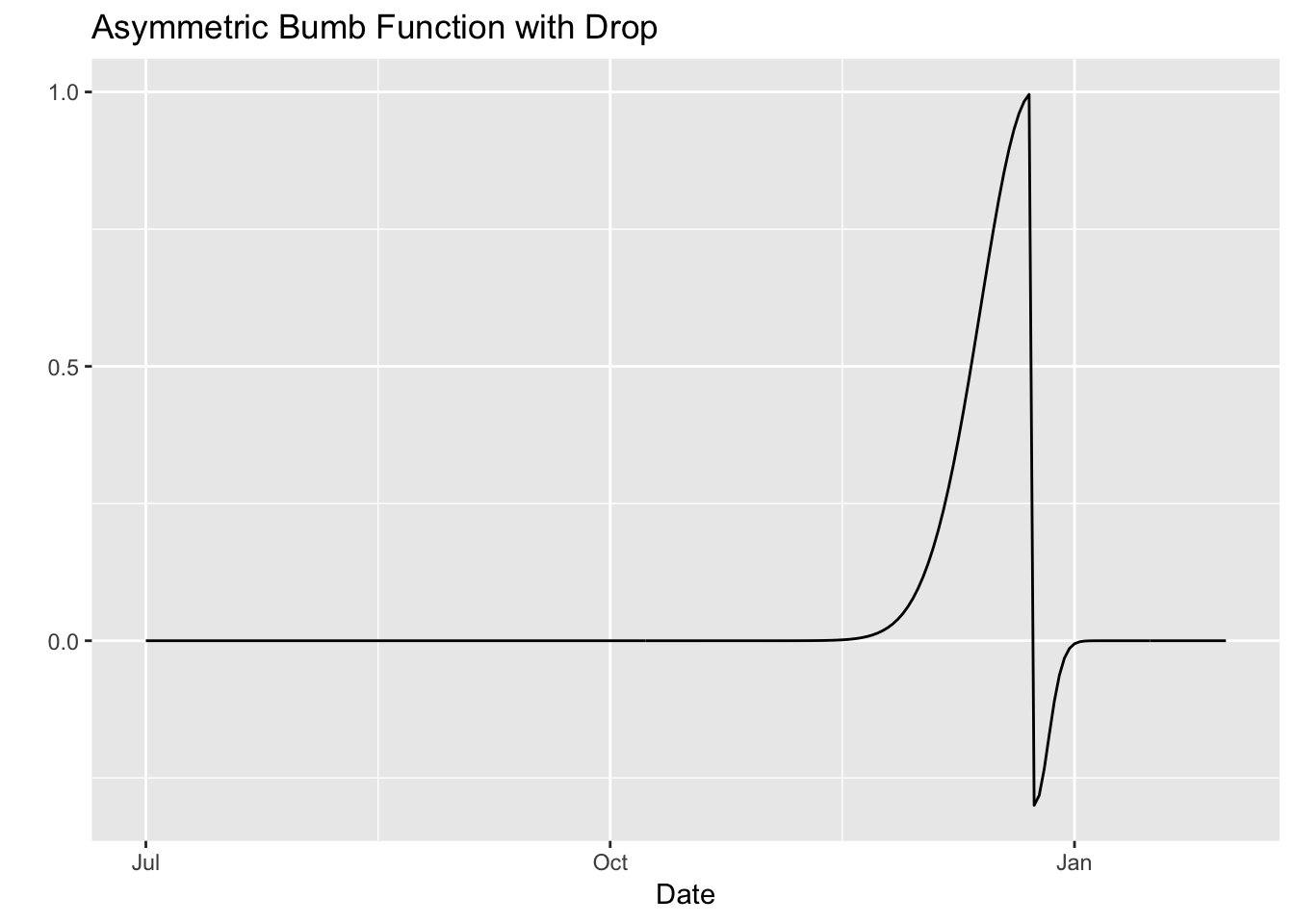
With Drop
df  %>%
  mutate(y =  asymmestric_bump_func(x = t,
                                    x_0 = as.Date("2017-12-24"),
                                    epsilon_minus = 15,
                                    epsilon_plus = 4,
                                    a_minus = 1,
                                    a_plus = 0.3,
                                    drop = TRUE)) %>%
  # Filter for visualization (zoom in).
  filter(t < "2018-02-01") %>%
  ggplot() +
  geom_line(mapping = aes(x = t, y = y)) +
  xlab("Date") +
  ylab("") +
  ggtitle(label = glue("Asymmetric Bumb Function with Drop"))