In this notebook we present an example of a regression model with time varying coefficients using Gaussian processes. In particular, we use a Hilbert space Gaussian process approximation in pymc to speed up the computations (see HSGP). We continue using the bikes dataset from the previous posts (Exploring Tools for Interpretable Machine Learning and Time-Varying Regression Coefficients via Gaussian Random Walk in PyMC). Please refer to those posts for more details on the dataset, EDA and base models. In essence, we are trying to model bike count rentals as a function of meteorological variables and seasonality. We are particularly interested in the marginal effect of temperature on bike rentals, which we expect to be non-linear.
Prepare Notebook
import arviz as az
import matplotlib.pyplot as plt
import numpy as np
import pandas as pd
import preliz as pz
import pymc as pm
import seaborn as sns

from pymc.gp.util import plot_gp_dist
from sklearn.preprocessing import MaxAbsScaler

plt.style.use("bmh")
plt.rcParams["figure.figsize"] = [12, 7]
plt.rcParams["figure.dpi"] = 100
plt.rcParams["figure.facecolor"] = "white"

%load_ext autoreload
%autoreload 2
%config InlineBackend.figure_format = "retina"
seed: int = sum(map(ord, "bikes"))
rng: np.random.Generator = np.random.default_rng(seed=seed)
Read Data
We read the data and create the date and eoys variables in the previous post.
data_path = "https://raw.githubusercontent.com/christophM/interpretable-ml-book/master/data/bike.csv"

raw_data_df = pd.read_csv(
    data_path,
    dtype={
        "season": "category",
        "mnth": "category",
        "holiday": "category",
        "weekday": "category",
        "workingday": "category",
        "weathersit": "category",
        "cnt": "int",
    },
)

data_df = raw_data_df.copy()

data_df["date"] = pd.to_datetime("2011-01-01") + data_df["days_since_2011"].apply(
    lambda z: pd.Timedelta(z, unit="D")
)

# end-of-year Gaussian bump
is_december = data_df["date"].dt.month == 12
eoy_mu = 25
eoy_sigma = 7
eoy_arg = (data_df["date"].dt.day - eoy_mu) / eoy_sigma
data_df["eoy"] = is_december * np.exp(-(eoy_arg**2))

data_df.info()
<class 'pandas.core.frame.DataFrame'>
RangeIndex: 731 entries, 0 to 730
Data columns (total 14 columns):
 #   Column           Non-Null Count  Dtype
---  ------           --------------  -----
 0   season           731 non-null    category
 1   yr               731 non-null    int64
 2   mnth             731 non-null    category
 3   holiday          731 non-null    category
 4   weekday          731 non-null    category
 5   workingday       731 non-null    category
 6   weathersit       731 non-null    category
 7   temp             731 non-null    float64
 8   hum              731 non-null    float64
 9   windspeed        731 non-null    float64
 10  cnt              731 non-null    int64
 11  days_since_2011  731 non-null    int64
 12  date             731 non-null    datetime64[ns]
 13  eoy              731 non-null    float64
dtypes: category(6), datetime64[ns](1), float64(4), int64(3)
memory usage: 51.3 KB
Prepare Data
We scale and one-hot encode the continuous and categorical variables, respectively.
target = "cnt"
target_scaled = f"{target}_scaled"

endog_scaler = MaxAbsScaler()
exog_scaler = MaxAbsScaler()


data_df[target_scaled] = endog_scaler.fit_transform(X=data_df[[target]])
data_df[["temp_scaled", "hum_scaled", "windspeed_scaled"]] = exog_scaler.fit_transform(
    X=data_df[["temp", "hum", "windspeed"]]
)
n = data_df.shape[0]
# target
cnt = data_df[target].to_numpy()
cnt_scaled = data_df[target_scaled].to_numpy()
# date feature
date = data_df["date"].to_numpy()
# model regressors
temp_scaled = data_df["temp_scaled"].to_numpy()
hum_scaled = data_df["hum_scaled"].to_numpy()
windspeed_scaled = data_df["windspeed_scaled"].to_numpy()
holiday_idx, holiday = data_df["holiday"].factorize(sort=True)
workingday_idx, workingday = data_df["workingday"].factorize(sort=True)
weathersit_idx, weathersit = data_df["weathersit"].factorize(sort=True)
t = data_df["days_since_2011"].to_numpy() / data_df["days_since_2011"].max()
eoy = data_df["eoy"].to_numpy()Model Structure
We model the bikes count through a StudentT likelihood (as an approximation as the bike counts are large integers). Now we describe the components of the model.
- For the categorical variables we use a
ZeroSumNormaldistribution as we have an intercept term and we are interested about the relative deviations. - For the continuous variables
temp,humandwindspeedwe useGaussian processesto model the time-variant coefficients. For a introduction to Gaussian processes you can see previous blog posts: Bayesian Regression as a Gaussian Process and An Introduction to Gaussian Process Regression.- The domain of definition of the Gaussian process is not the
datevariable bur rather thetemp,humandwindspeedvariables respectively. This is because we want to model the effect of the continuous variables on the bike count (I must admit this was a Clever Hans Effect 🙈). - We use
ExpQuadkernels. - As the data is scaled we use a single length-scale and amplitudes for all the variables (I tried a hierarchical model but it did not make much difference).
- Instead of adding manually a linear trend, we use another Gaussian process to model a latent background trend.
- We use a
HSGPapproximation to speed up the computations. Please check the video PyMCon Web Series - Introduction to Hilbert Space GPs in PyMC by Bill Engels for a great introduction to the topic. The original paper Hilbert space methods for reduced-rank Gaussian process regression is also a great resource.
- The domain of definition of the Gaussian process is not the
coords = {
    "date": date,
    "holiday": holiday,
    "workingday": workingday,
    "weathersit": weathersit,
}


with pm.Model(coords=coords) as model:
    # --- priors ---
    ls_latent_params = pm.find_constrained_prior(
        distribution=pm.InverseGamma,
        lower=0.05,
        upper=0.5,
        init_guess={"alpha": 2, "beta": 0.2},
        mass=0.95,
    )
    ls_latent = pm.InverseGamma(name="ls_latent", **ls_latent_params)
    amplitude_latent = pm.Exponential(name="amplitude_latent", lam=1 / 0.5)
    cov_latent = amplitude_latent**2 * pm.gp.cov.ExpQuad(input_dim=1, ls=ls_latent)
    gp_latent = pm.gp.HSGP(m=[10], c=1.3, cov_func=cov_latent)
    f_latent = gp_latent.prior(name="f_latent", X=t[:, None], dims="date")

    ls_params = pm.find_constrained_prior(
        distribution=pm.InverseGamma,
        lower=0.1,
        upper=0.7,
        init_guess={"alpha": 2, "beta": 0.5},
        mass=0.95,
    )
    ls = pm.InverseGamma(name="ls", **ls_params)

    amplitude = pm.Exponential(name="amplitude", lam=1 / 0.5)

    cov_temp = amplitude**2 * pm.gp.cov.ExpQuad(input_dim=1, ls=ls)
    gp_temp = pm.gp.HSGP(m=[20], c=1.3, cov_func=cov_temp)
    b_temp = gp_temp.prior(name="b_temp", X=temp_scaled[:, None], dims="date")

    cov_hum = amplitude**2 * pm.gp.cov.ExpQuad(input_dim=1, ls=ls)
    gp_hum = pm.gp.HSGP(m=[20], c=1.3, cov_func=cov_hum)
    b_hum = gp_hum.prior(name="b_hum", X=hum_scaled[:, None], dims="date")

    cov_windspeed = amplitude**2 * pm.gp.cov.ExpQuad(input_dim=1, ls=ls)
    gp_windspeed = pm.gp.HSGP(m=[20], c=1.3, cov_func=cov_windspeed)
    b_windspeed = gp_hum.prior(
        name="b_windspeed", X=windspeed_scaled[:, None], dims="date"
    )

    b_holiday = pm.ZeroSumNormal(name="b_holiday", sigma=1, dims="holiday")
    b_workingday = pm.ZeroSumNormal(name="b_workingday", sigma=1, dims="workingday")
    b_weathersit = pm.ZeroSumNormal(name="b_weathersit", sigma=1, dims="weathersit")
    b_eoy = pm.Normal(name="b_eoy", mu=0, sigma=1)
    nu = pm.Gamma(name="nu", alpha=4, beta=1)
    sigma = pm.Exponential(name="sigma", lam=1 / 0.2)

    # --- model parametrization ---
    mu = pm.Deterministic(
        name="mu",
        var=(
            f_latent
            + b_temp * temp_scaled
            + b_hum * hum_scaled
            + b_windspeed * windspeed_scaled
            + b_holiday[holiday_idx]
            + b_workingday[workingday_idx]
            + b_weathersit[weathersit_idx]
            + b_eoy * eoy
        ),
        dims="date",
    )

    # --- likelihood ---
    likelihood = pm.StudentT(
        name="likelihood", mu=mu, nu=nu, sigma=sigma, dims="date", observed=cnt_scaled
    )


pm.model_to_graphviz(model=model)

Prior Predictive Checks
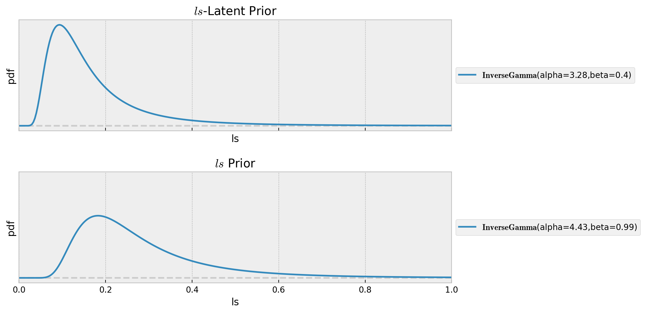
Before sampling from the prior distribution, we can visualize the prior for the ls parameter:
ls_latent_params = pm.find_constrained_prior(
    distribution=pm.InverseGamma,
    lower=0.05,
    upper=0.5,
    init_guess={"alpha": 2, "beta": 0.2},
    mass=0.95,
)

ls_params = pm.find_constrained_prior(
    distribution=pm.InverseGamma,
    lower=0.1,
    upper=0.7,
    init_guess={"alpha": 2, "beta": 0.5},
    mass=0.95,
)

fig, ax = plt.subplots(
    nrows=2, ncols=1, figsize=(8, 5), sharex=True, sharey=True, layout="constrained"
)
fig.tight_layout(h_pad=4)
pz.InverseGamma(**ls_latent_params).plot_pdf(ax=ax[0])
ax[0].set(title=r"$ls$-Latent Prior", xlim=(0, 1), xlabel="ls", ylabel="pdf")
pz.InverseGamma(**ls_params).plot_pdf(ax=ax[1])
ax[1].set(title=r"$ls$ Prior", xlim=(0, 1), xlabel="ls", ylabel="pdf")
with model:
    prior_predictive = pm.sample_prior_predictive(samples=500, random_seed=rng)
fig, ax = plt.subplots()
az.plot_hdi(
x=date,
y=prior_predictive["prior_predictive"]["likelihood"],
color="C0",
smooth=False,
hdi_prob=0.94,
fill_kwargs={"alpha": 0.4, "label": "$94\%$ HDI"},
ax=ax,
)
az.plot_hdi(
x=date,
y=prior_predictive["prior_predictive"]["likelihood"],
color="C0",
smooth=False,
hdi_prob=0.5,
fill_kwargs={"alpha": 0.6, "label": "$50\%$ HDI"},
ax=ax,
)
ax.plot(date, cnt_scaled, color="black", label=target_scaled)
ax.legend(loc="upper left")
ax.set(
title="Prior Predictive",
xlabel="date",
ylabel=target_scaled,
)
The model specification looks reasonable.
Model Fit
Now we fit the model:
with model:
    idata = pm.sample(
        target_accept=0.9,
        draws=4_000,
        chains=5,
        nuts_sampler="numpyro",
        random_seed=rng,
    )
    posterior_predictive = pm.sample_posterior_predictive(trace=idata, random_seed=rng)
idata["sample_stats"]["diverging"].sum().item()
0Observe that the model samples quite fast given the fact it has \(4\) Gaussian processes and more than \(7000\) observations. We can now look into the posterior distributions of the coefficients and diagnostics.
var_names = [
    "ls_latent",
    "ls",
    "amplitude_latent",
    "amplitude",
    "b_holiday",
    "b_workingday",
    "b_weathersit",
    "b_eoy",
    "sigma",
    "nu",
]

az.summary(data=idata, var_names=var_names)
| mean | sd | hdi_3% | hdi_97% | mcse_mean | mcse_sd | ess_bulk | ess_tail | r_hat | |
|---|---|---|---|---|---|---|---|---|---|
| ls_latent | 0.140 | 0.025 | 0.091 | 0.179 | 0.001 | 0.000 | 3508.0 | 1482.0 | 1.0 |
| ls | 0.401 | 0.054 | 0.300 | 0.504 | 0.001 | 0.000 | 10246.0 | 12861.0 | 1.0 |
| amplitude_latent | 0.275 | 0.093 | 0.135 | 0.447 | 0.001 | 0.001 | 6641.0 | 9852.0 | 1.0 |
| amplitude | 0.279 | 0.096 | 0.140 | 0.457 | 0.001 | 0.001 | 9894.0 | 11656.0 | 1.0 |
| b_holiday[HOLIDAY] | -0.024 | 0.007 | -0.038 | -0.011 | 0.000 | 0.000 | 42504.0 | 15211.0 | 1.0 |
| b_holiday[NO HOLIDAY] | 0.024 | 0.007 | 0.011 | 0.038 | 0.000 | 0.000 | 42504.0 | 15211.0 | 1.0 |
| b_workingday[NO WORKING DAY] | -0.007 | 0.003 | -0.012 | -0.002 | 0.000 | 0.000 | 37599.0 | 15807.0 | 1.0 |
| b_workingday[WORKING DAY] | 0.007 | 0.003 | 0.002 | 0.012 | 0.000 | 0.000 | 37599.0 | 15807.0 | 1.0 |
| b_weathersit[GOOD] | 0.075 | 0.009 | 0.059 | 0.091 | 0.000 | 0.000 | 22242.0 | 16807.0 | 1.0 |
| b_weathersit[MISTY] | 0.040 | 0.008 | 0.025 | 0.055 | 0.000 | 0.000 | 21873.0 | 16660.0 | 1.0 |
| b_weathersit[RAIN/SNOW/STORM] | -0.115 | 0.015 | -0.143 | -0.087 | 0.000 | 0.000 | 22499.0 | 15907.0 | 1.0 |
| b_eoy | -0.192 | 0.021 | -0.230 | -0.151 | 0.000 | 0.000 | 28523.0 | 14790.0 | 1.0 |
| sigma | 0.049 | 0.003 | 0.044 | 0.053 | 0.000 | 0.000 | 16243.0 | 14110.0 | 1.0 |
| nu | 3.221 | 0.445 | 2.437 | 4.077 | 0.003 | 0.002 | 24273.0 | 15672.0 | 1.0 |
axes = az.plot_trace(
    data=idata,
    var_names=var_names,
    compact=True,
    kind="rank_bars",
    backend_kwargs={"figsize": (12, 15), "layout": "constrained"},
)
plt.gcf().suptitle("Time-Varying Coefficient Model - Trace", fontsize=16)
az.plot_forest(
    data=idata,
    var_names=[v for v in var_names if v != "nu"],
    combined=True,
    figsize=(12, 8),
    ess=True,
    r_hat=True,
)
fig, ax = plt.subplots(
    nrows=2, ncols=1, figsize=(10, 6), sharex=True, sharey=True, layout="constrained"
)
fig.tight_layout(h_pad=5)
pz.InverseGamma(**ls_latent_params).plot_pdf(ax=ax[0])
az.plot_posterior(
    data=idata, var_names=["ls_latent"], color="C1", label="posterior", ax=ax[0]
)
ax[0].set(
    title=r"$ls$-Latent Prior vs Posterior", xlim=(0, 1), xlabel="ls", ylabel="pdf"
)
pz.InverseGamma(**ls_params).plot_pdf(ax=ax[1])
az.plot_posterior(data=idata, var_names=["ls"], color="C1", label="posterior", ax=ax[1])
ax[1].set(title=r"$ls$ Prior vs Posterior", xlim=(0, 1), xlabel="ls", ylabel="pdf")

The results look good and the coefficients for the categorical variables make a lot of sense!
Posterior Predictive Checks
fig, ax = plt.subplots()
az.plot_hdi(
    x=date,
    y=posterior_predictive["posterior_predictive"]["likelihood"],
    color="C0",
    smooth=False,
    hdi_prob=0.94,
    fill_kwargs={"alpha": 0.4, "label": "$94\%$ HDI"},
    ax=ax,
)
az.plot_hdi(
    x=date,
    y=posterior_predictive["posterior_predictive"]["likelihood"],
    color="C0",
    smooth=False,
    hdi_prob=0.5,
    fill_kwargs={"alpha": 0.6, "label": "$50\%$ HDI"},
    ax=ax,
)
ax.plot(date, cnt_scaled, color="black", label=target_scaled)
ax.legend(loc="upper left")
ax.set(
    title="Posterior Predictive",
    xlabel="date",
    ylabel=target_scaled,
)

ax = az.plot_ppc(
    data=posterior_predictive,
    observed_rug=True,
    random_seed=seed,
)
ax.set(
    title="Posterior Predictive Check",
    xlabel="likelihood (bike counts scaled)",
    xlim=(-0.5, 1.5),
)

Model Components Deep Dive
Now we examine the Gaussian processes components of the model in more detail.
Latent Trend
We start by looking into the latent trend components:
f_latent_samples = az.extract(data=idata, var_names=["f_latent"]).transpose(
    "sample", ...
)

fig, ax = plt.subplots()
plot_gp_dist(
    ax=ax,
    samples=f_latent_samples,
    x=date,
    palette="viridis_r",
)
ax.set(title="Latent Process - Posterior Predictive", xlabel="date", ylabel=None)

We see that this latent process is very smooth and seems to be capturing the global trend of the bike rentals.
Temperature
We now focus on the variable temp, which is the one we are most interested in.
b_temp_samples = az.extract(data=idata, var_names=["b_temp"]).transpose("sample", ...)

fig, ax = plt.subplots()
plot_gp_dist(
    ax=ax,
    samples=b_temp_samples,
    x=data_df["temp"].to_numpy(),
    palette="viridis_r",
)
sns.rugplot(x=data_df["temp"], color="black", ax=ax)
ax.axhline(y=0.0, color="gray", linestyle="--")
ax.set(
    title="Temperature Coefficient - Posterior Predictive", xlabel="temp", ylabel=None
)

The time-varying effect is similar to the one obtained in the previous post Time-Varying Regression Coefficients via Gaussian Random Walk in PyMC. In this case the estimation is less noisy, in particular for lower temperatures. This might be due to the fact that we are using a more flexible trend component. Let’s look now into the development over time:
fig, ax = plt.subplots()
plot_gp_dist(
    ax=ax,
    samples=b_temp_samples,
    x=date,
    palette="viridis_r",
)
ax.set(
    title="Temperature Coefficient over Time - Posterior Predictive",
    xlabel="date",
    ylabel=None,
)
We see how the temperature effect drops significantly during the summer months, while relatively stable during the rest of the year.
Let’s compare the latent trend and the temperature effects:
fig, ax = plt.subplots(figsize=(12, 7))
sns.lineplot(x=date, y=cnt, color="black", ax=ax)
plot_gp_dist(
    ax=ax,
    samples=endog_scaler.inverse_transform(X=f_latent_samples),
    x=date,
    palette="viridis_r",
)
plot_gp_dist(
    ax=ax,
    samples=endog_scaler.inverse_transform(X=b_temp_samples * temp_scaled[None, ...]),
    x=date,
    palette="Spectral_r",
)
ax.set(title="Latent Process - Posterior Predictive", xlabel="date", ylabel=None)
Humidity
b_hum_samples = az.extract(data=idata, var_names=["b_hum"]).transpose("sample", ...)

fig, ax = plt.subplots()
plot_gp_dist(
    ax=ax,
    samples=b_hum_samples,
    x=data_df["hum"].to_numpy(),
    palette="viridis_r",
)
sns.rugplot(x=data_df["hum"], color="black", ax=ax)
ax.axhline(y=0.0, color="gray", linestyle="--")
ax.set(title="Humidity Coefficient - Posterior Predictive", xlabel="hum", ylabel=None)

This variable seems to have a decreasing effect on the bike rentals. It even changes sign for humidity values higher than \(0.8\).
fig, ax = plt.subplots()
plot_gp_dist(
    ax=ax,
    samples=b_hum_samples,
    x=date,
    palette="viridis_r",
)
ax.set(
    title="Humidity Coefficient over Time - Posterior Predictive",
    xlabel="date",
    ylabel=None,
)
Wind Speed
b_windspeed_samples = az.extract(data=idata, var_names=["b_windspeed"]).transpose(
    "sample", ...
)

fig, ax = plt.subplots()
plot_gp_dist(
    ax=ax,
    samples=b_windspeed_samples,
    x=data_df["windspeed"].to_numpy(),
    palette="viridis_r",
)
sns.rugplot(x=data_df["windspeed"], color="black", ax=ax)
ax.axhline(y=0.0, color="gray", linestyle="--")
ax.set(
    title="Wind Speed Coefficient - Posterior Predictive",
    xlabel="windspeed",
    ylabel=None,
)

The winds speed coefficient looks flat and negative.
fig, ax = plt.subplots()
plot_gp_dist(
    ax=ax,
    samples=b_windspeed_samples,
    x=date,
    palette="viridis_r",
)
ax.set(
    title="Wind Speed Coefficient over Time - Posterior Predictive",
    xlabel="date",
    ylabel=None,
)
Remark: Observe that the learned time-varying coefficients are very similar to the partial dependency plots of the tree-based ensemble model presented in the post Exploring Tools for Interpretable Machine Learning.
Effects Original Scale
We can transform back the time-varying effects to the original scale (see How to vectorize an scikit-learn transformer over a numpy array?)
stacked_samples = np.moveaxis(
    a=np.stack(
        [
            b_temp_samples.to_numpy(),
            b_hum_samples.to_numpy(),
            b_windspeed_samples.to_numpy(),
        ],
        axis=1,
    ),
    source=1,
    destination=2,
)

vectorized_exog_scaler = np.vectorize(
    pyfunc=exog_scaler.transform,
    excluded=[1, 2],
    signature="(m, n) -> (m, n)",
)

stacked_samples_transformed = vectorized_exog_scaler(stacked_samples)
stacked_samples_transformed.shape
(20000, 731, 3)temp_samples_original_scale = endog_scaler.inverse_transform(
stacked_samples_transformed[:, :, 0]
)
fig, ax = plt.subplots()
az.plot_hdi(
x=data_df["temp"].to_numpy(),
y=temp_samples_original_scale,
hdi_prob=0.94,
color="C0",
fill_kwargs={"alpha": 0.4, "label": "$94\%$ HDI"},
ax=ax,
)
az.plot_hdi(
x=data_df["temp"].to_numpy(),
y=temp_samples_original_scale,
hdi_prob=0.5,
color="C0",
fill_kwargs={"alpha": 0.6, "label": "$50\%$ HDI"},
ax=ax,
)
ax.axhline(
y=109.1, # <- from baseline model from previous post
color="C1",
linestyle="--",
label="base model posterior predictive mean",
)
sns.rugplot(x=data_df["temp"], color="black", alpha=0.5, ax=ax)
ax.axhline(y=0.0, color="gray", linestyle="--")
ax.legend(loc="upper left")
ax.set(
title="Temperature Coefficient (Original Scale) - Posterior Predictive",
xlabel="temp",
ylabel=None,
)
hum_samples_original_scale = endog_scaler.inverse_transform(
    stacked_samples_transformed[:, :, 1]
)


fig, ax = plt.subplots()
az.plot_hdi(
    x=data_df["hum"].to_numpy(),
    y=hum_samples_original_scale,
    hdi_prob=0.94,
    color="C0",
    fill_kwargs={"alpha": 0.4, "label": "$94\%$ HDI"},
    ax=ax,
)
az.plot_hdi(
    x=data_df["hum"].to_numpy(),
    y=hum_samples_original_scale,
    hdi_prob=0.5,
    color="C0",
    fill_kwargs={"alpha": 0.6, "label": "$50\%$ HDI"},
    ax=ax,
)
sns.rugplot(x=data_df["hum"], color="black", alpha=0.5, ax=ax)
ax.axhline(y=0.0, color="gray", linestyle="--")
ax.legend(loc="upper left")
ax.set(
    title="Humidity Coefficient (Original Scale) - Posterior Predictive",
    xlabel="hum",
    ylabel=None,
)

windspeed_samples_original_scale = endog_scaler.inverse_transform(
    stacked_samples_transformed[:, :, 2]
)


fig, ax = plt.subplots()
az.plot_hdi(
    x=data_df["windspeed"].to_numpy(),
    y=windspeed_samples_original_scale,
    hdi_prob=0.94,
    color="C0",
    fill_kwargs={"alpha": 0.4, "label": "$94\%$ HDI"},
    ax=ax,
)
az.plot_hdi(
    x=data_df["windspeed"].to_numpy(),
    y=windspeed_samples_original_scale,
    hdi_prob=0.5,
    color="C0",
    fill_kwargs={"alpha": 0.6, "label": "$50\%$ HDI"},
    ax=ax,
)
sns.rugplot(x=data_df["windspeed"], color="black", alpha=0.5, ax=ax)
ax.axhline(y=0.0, color="gray", linestyle="--")
ax.legend(loc="upper left")
ax.set(
    title="Wind Speed Coefficient (Original Scale) - Posterior Predictive",
    xlabel="windspeed",
    ylabel=None,
)

The results are consistent with the curves obtained in the post Time-Varying Regression Coefficients via Gaussian Random Walk in PyMC using a GaussianRandomWalk. Still, I found using Gaussian processes more intuitive and flexible (specially because the Hilbert space approximation).