Nowadays social media generates a vast amount of raw data (text, images, videos, etc). It is a very interesting challenge to discover techniques to get insights on the content and development of social media data. In addition, as a fundamental component of the analysis, it is important to find ways of communicating the results, i.e. data visualization. In this post I want to present a small case study where I analyze Twitter text data. The aim is not to give a complete analysis (as it would require many interations), but rather to describe how to to start. The emphasis of this post is in the data manipulation and data visualization. In particular, I describe how networks (graphs) can be used as data structures to describe text relations (some measure of pairwise count occurrences).
The topic I chose to run the analysis is the Colombian peace agreement referendum (Plebiscito), celebrated on 2016-10-02. You can find more information about it here. In a previous post I described how to get (scraping) the referendum results data per town.
The analysis is done in R and it is mainly motivated by the techniques presented in the book Text Mining with R.
1. Data Source
The data for the analysis consists of ~ 33.7K Twitter posts, generated between the 2016-10-02 and 2016-10-03, containing relevant hashtags related the the Plebiscito. The data is freely available at Plebicito Tweets 2016 on the website data.world. The raw data was collected (using Twitter API) by Victor Ramirez. On his website you can find the data gathering description and a brief initial analysis. The hashtags tracked were:
- #HoyVotoSi, #SiALaPaz, #YoVotoSi
- #HoyVotoNo, #SoyColombiaNO, #YoVotoNo
Remark: No user-specific data was used. All account references on the tweets were deleted.
2. Prepare Notebook
Let us load the required libraries.
# Data Wrangling and Visualization
library(glue)
library(cowplot)
library(magrittr)
library(plotly)
library(tidyverse)
library(widyr)
# Date & Time Manipulation.
library(hms)
library(lubridate)
# Text Mining
library(tidytext)
library(tm)
library(wordcloud)
# Network Analysis
library(igraph)
# Network Visualization (D3.js)
library(networkD3)
# Set notebook directory.
MAIN.DIR <- here::here()
3. Read Data
# Set file path.
file.name <- glue('{MAIN.DIR}/static/data/plebiscito.json')

# Read each line.
tweets.raw.list <- map(
  .x = read_lines(file = file.name),
  .f = rjson::fromJSON
)

# Parse subset of the data into a tibble.
tweets.raw.df <- tweets.raw.list %>%
  map_df(.f = ~ data.frame(
    # Select non-user related data.
    ID = .x$id_str,
    Created_At = .x$created_at,
    Text = .x$text,
    stringsAsFactors = FALSE
    )
  ) %>%
  as_tibble()

tweets.raw.df %>%
  # We  do not want to display accounts.
  filter(!str_detect(string = Text, pattern = '@')) %>%
  head()
## # A tibble: 6 x 3
## ID Created_At Text
## <chr> <chr> <chr>
## 1 78261639629… Sun Oct 02 16:21:03 … "#HappySunday #FelizDomingo #DomingoDeGan…
## 2 78261640341… Sun Oct 02 16:21:05 … "Por una Colombia diferente. #VotoSiALaPaz…
## 3 78261640705… Sun Oct 02 16:21:06 … "Me voy acercando a mi puesto de votación …
## 4 78261640845… Sun Oct 02 16:21:06 … "Hoy todos los que vamos por el SI, alegre…
## 5 78261641049… Sun Oct 02 16:21:07 … "#HoyVotoSi\nPor un gran futuro para Colom…
## 6 78261641683… Sun Oct 02 16:21:08 … "#VotoSiALaPaz #HoyVotoSi #VotacionesSegur…Let us see the structure of this tibble.
tweets.raw.df %>% glimpse()## Observations: 33,762
## Variables: 3
## $ ID <chr> "782616396299730944", "782616402310094849", "7826164034174…
## $ Created_At <chr> "Sun Oct 02 16:21:03 +0000 2016", "Sun Oct 02 16:21:05 +00…
## $ Text <chr> "#HappySunday #FelizDomingo #DomingoDeGanarSeguidores #Si…We parse the Created_At column into a date format. Note that in the raw file it has type character.
tweets.raw.df %>%
  slice(1:4) %>%
  pull(Created_At)
## [1] "Sun Oct 02 16:21:03 +0000 2016" "Sun Oct 02 16:21:05 +0000 2016"
## [3] "Sun Oct 02 16:21:05 +0000 2016" "Sun Oct 02 16:21:06 +0000 2016"tweets.raw.df %<>%
mutate(
Created_At = Created_At %>%
# Remove zeros.
str_remove_all(pattern = '\\+0000') %>%
# Parse date.
parse_date_time(orders = '%a %b %d %H%M%S %Y')
)
tweets.raw.df %>%
filter(!str_detect(string = Text, pattern = '@')) %>%
head()## # A tibble: 6 x 3
## ID Created_At Text
## <chr> <dttm> <chr>
## 1 782616396299… 2016-10-02 16:21:03 "#HappySunday #FelizDomingo #DomingoDeGana…
## 2 782616403417… 2016-10-02 16:21:05 "Por una Colombia diferente. #VotoSiALaPaz …
## 3 782616407058… 2016-10-02 16:21:06 "Me voy acercando a mi puesto de votación y…
## 4 782616408458… 2016-10-02 16:21:06 "Hoy todos los que vamos por el SI, alegres…
## 5 782616410493… 2016-10-02 16:21:07 "#HoyVotoSi\nPor un gran futuro para Colomb…
## 6 782616416835… 2016-10-02 16:21:08 "#VotoSiALaPaz #HoyVotoSi #VotacionesSegura…4. Timeline Analysis
As the Created_At column makes reference to the UTC time, we neet to substract 5 hours from it to get the Colombian time.
# We substract seconds, that is why we need three factors.
tweets.raw.df %<>%
  mutate(Created_At = Created_At - 5*60*60)
Let us compute the time range:
tweets.raw.df %>% pull(Created_At) %>% min()## [1] "2016-10-02 11:21:03 UTC"tweets.raw.df %>% pull(Created_At) %>% max()## [1] "2016-10-03 17:43:47 UTC"We see that the time frame covered by this data set is essentially the day and the day after the referendum.
We create a new variable which “forgets” the seconds of Create_At column.
tweets.raw.df %<>%
  mutate(Created_At_Round = Created_At %>% round(units = 'mins') %>% as.POSIXct())
We now plot the time series of tweets count per minute.
plt <- tweets.raw.df %>%
  count(Created_At_Round) %>%
  ggplot(mapping = aes(x = Created_At_Round, y = n)) +
    theme_light() +
    geom_line() +
    xlab(label = 'Date') +
    ylab(label = NULL) +
    ggtitle(label = 'Number of Tweets per Minute')

plt %>% ggplotly()
There is an interesting peak at around 2016-10-02 19:28:00, which is essentially when the referendum results where known. Let us have a look at some tweets after durinng this peak:
results.time <- as.POSIXct(x = '2016-10-02 19:28:00')

tweets.raw.df %>%
  filter(Created_At_Round > results.time ) %>%
  select(Text) %>%
  filter(!str_detect(string = Text, pattern = '@')) %>%
  pull(Text) %>%
  head(20)
## [1] "Espero que todos los que votaron por el NO mañana mismo se vayan para el monte con su rifle... \U0001f611\U0001f611\n\n#ColombiaDecide #YoVotoSi"
## [2] "Colombia quiere paz, pero no con tanta impunidad y beneficios. Colombia despertó!! \U0001f64f\U0001f44f\U0001f4aa. #SoyColombiaNO"
## [3] "Re-coherentes los hptas. https://t.co/UbUeqsUiD6"
## [4] "Y Colombia botó su voto dejando ganar el no... #ColombiaDecide #HoyVotoSi"
## [5] "Ay martincito...sos una caricatura! Que pesar! https://t.co/0kokGc52w2"
## [6] "En las zonas golpeadas por la guerra gano el #SiALaPaz, siento #dolor de #patria #ColombiaDecide #pais #sinmemoria."
## [7] "Ganamos Colombia #ColombiaDecide no lo puedo creer! #sialapaz #noalplebiscito"
## [8] "Sé que he cumplido con mi deber, tristemente todos hemos perdido, llamo a la unidad porque en este país cabemos todos.\n#SiALaPAZ ¿cuándo?"
## [9] "Jaja! https://t.co/9HlsYeT6w7"
## [10] "Deberían priorizar los resultados de los lugares afectados por la guerra. Dijeron #SiaLAPaz , no es justo que otros decidan por ellos."
## [11] "Día triste para Colombia gana el no \ntodo este tiempo fue en vano #SiALaPaz https://t.co/bq36CRvvvx"
## [12] "Tristesa #SiaLAPazenColombia #SiALaPaz https://t.co/r5yZDFLTC1"
## [13] "Ganó el #VotoNo #ColombiaDecide\nEs clave saber qué va a pasar con el proceso de paz y saber si van a renegociar lo… https://t.co/6DqGBz20XF"
## [14] "#ColombiaDecide #HoyVotoSi \nVivo en el país más ignorante del mundo,\nQue lastima pueblo!"
## [15] "#DolordePatria \n#HoyVotoSi #VotoSiSinSerSantista https://t.co/CVXZCBNNwx"
## [16] "el que mas ayudo al #VotoNo fue Mateo, al no poder salir la gente a votar en la costa, bastión de la Mermelada y compra de votos de Santos."
## [17] "76. Cada cartucho de fusil cuesta $ 1.040 y este dispara 300 cartuchos por minuto, lo que cuestan 900 huevos… https://t.co/NtbpwCZFD4"
## [18] "Brexit otra vez y los más cuerdos parecen los de las FARC . Incertidumbre para los colombianos #SiALaPaz https://t.co/3wYYyU6wC2"
## [19] "#ColombiaDecide\nLa decepción electoral debe fortalecernos para desde mañana mismo seguir generando conciencia en favor del pueblo.\n#SiALaPaz"
## [20] "Porque será que nunca hemos podido aprender a perdonar? Porque será que nos puede el odio y la ignorancia?? #ColombiaDecide #SiALaPaz"Indeed, the comments reflect the reactions around the referendum results.
5. Text Normalization
We want to clean and normalize the text for the analysis. We are mainly interested in the content of the tweets, not the hashtags or accounts.
tweets.df <- tweets.raw.df %>%
# Remove column.
select(- Created_At) %>%
# Convert to lowercase.
mutate(Text = Text %>% str_to_lower) %>%
# Remove unwanted characters.
mutate(Text= Text %>% str_remove_all(pattern = '\\n')) %>%
mutate(Text = Text %>% str_remove_all(pattern = '&')) %>%
mutate(Text = Text %>% str_remove_all(pattern = 'https://t.co/[a-z,A-Z,0-9]*')) %>%
mutate(Text = Text %>% str_remove_all(pattern = 'http://t.co/[a-z,A-Z,0-9]*')) %>%
mutate(Text = Text %>% str_remove_all(pattern = 'https')) %>%
mutate(Text = Text %>% str_remove_all(pattern = 'http')) %>%
# Remove hashtags.
mutate(Text = Text %>% str_remove_all(pattern = '#[a-z,A-Z]*')) %>%
# Remove accounts.
mutate(Text = Text %>% str_remove_all(pattern = '@[a-z,A-Z]*')) %>%
# Remove retweets.
mutate(Text = Text %>% str_remove_all(pattern = 'rt [a-z,A-Z]*: ')) %>%
mutate(Text = Text %>% str_remove(pattern = '^(rt)')) %>%
mutate(Text = Text %>% str_remove_all(pattern = '\\_'))
# Replace accents.
replacement.list <- list('á' = 'a', 'é' = 'e', 'í' = 'i', 'ó' = 'o', 'ú' = 'u')
tweets.df %<>%
mutate(Text = chartr(old = names(replacement.list) %>% str_c(collapse = ''),
new = replacement.list %>% str_c(collapse = ''),
x = Text))In addition, we convert out text into a corpus to use the tm library.
corpus <-  Corpus(x = VectorSource(x = tweets.df$Text))

tweets.text <- corpus %>%
  tm_map(removePunctuation) %>%
  tm_map(removeNumbers) %>%
  tm_map(removeWords, stopwords('spanish')) %>%
  tm_map(PlainTextDocument) # %>%
  # We could also use stemming by uncommenting the folowing line.
  # tm_map(stemDocument, 'spanish')

# Recover data into original tibble.
tweets.df %<>% mutate(Text = tweets.text[[1]]$content)
We now want to extract only the hashtags of each tweet. We implement a function for this purpose.
GetHashtags <- function(tweet) {

  hashtag.vector <- str_extract_all(string = tweet, pattern = '#\\S+', simplify = TRUE) %>%
    as.character()

  hashtag.string <- NA

  if (length(hashtag.vector) > 0) {

    hashtag.string <- hashtag.vector %>% str_c(collapse = ', ')

  }

  return(hashtag.string)
}
And apply it to our data:
hashtags.df <- tibble(
  Hashtags = tweets.raw.df$Text %>% map_chr(.f = ~ GetHashtags(tweet = .x))
)

hashtags.df %>% head()
## # A tibble: 6 x 1
## Hashtags
## <chr>
## 1 #HappySunday, #FelizDomingo, #DomingoDeGanarSeguidores, #SiaLAPazenColombia, …
## 2 #SiALaPaz, #PlebiscitoPorLaPaz
## 3 #VotoSiALaPaz, #VotoSi, #HoyVotoSi
## 4 #HoyVotoSi
## 5 #HoyVotoSi
## 6 #HoyVotoSi, #SialaPaz, #SíaLAPazenColombia, #FelizDomingoWe merge these data frames together.
tweets.df %<>% bind_cols(hashtags.df) Finally, let us split the data before and after the results of the referendum are known, i.e. we split the Created_At_Round column with respect to the results.time.
# "m" will represent before. results.time.
tweets.m.df <- tweets.df %>%
  filter(Created_At_Round < results.time) %>%
  select(ID, Text)

# "p" will represent after results.time.
tweets.p.df <- tweets.df %>%
  filter(Created_At_Round >= results.time) %>%
  select(ID, Text)
6. Words Count
6.1 Tweets
We begin by counting the most popular words in the tweets.
# Remove the shortcut 'q' for 'que'.
extra.stop.words <- c('q')

stopwords.df <- tibble(
  word = c(stopwords(kind = 'es'),
          # We have some tweets in english.
           stopwords(kind = 'en'),
           extra.stop.words)
  )

words.df <- tweets.df %>%
  unnest_tokens(input = Text, output = word) %>%
  anti_join(y = stopwords.df, by = 'word')

word.count <- words.df %>% count(word, sort = TRUE)

word.count %>% head(10)
## # A tibble: 10 x 2
## word n
## <chr> <int>
## 1 si 7642
## 2 paz 6166
## 3 colombia 4131
## 4 pais 3577
## 5 hoy 3477
## 6 llenos 3399
## 7 mas 3180
## 8 guerra 2709
## 9 colombianos 2459
## 10 voto 2086We can visualize these counts in a bar plot.
plt <- word.count %>%
# Set count threshold.
filter(n > 700) %>%
mutate(word = reorder(word, n)) %>%
ggplot(aes(x = word, y = n)) +
theme_light() +
geom_col(fill = 'black', alpha = 0.8) +
xlab(NULL) +
coord_flip() +
ggtitle(label = 'Top Word Count')
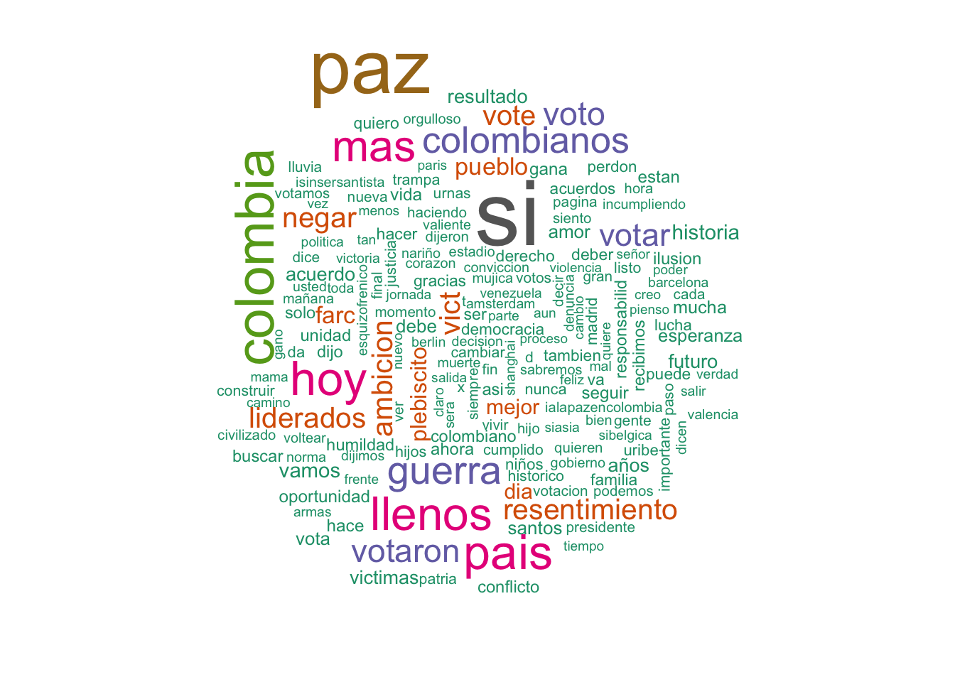
plt %>% ggplotly()Another popular method to visualize word count data is through a word cloud.
wordcloud(
  words = word.count$word,
  freq = word.count$n,
  min.freq = 200,
  colors = brewer.pal(8, 'Dark2')
)
We can do the same for the split data:
# Before results.
words.m.df <- tweets.m.df %>%
  unnest_tokens(input = Text, output = word) %>%
  anti_join(y = stopwords.df, by = 'word')

word.count.m <- words.m.df %>% count(word, sort = TRUE)

plt.m <- word.count.m %>%
  filter(n > 500) %>%
  mutate(word = reorder(word, n)) %>%
  ggplot(aes(x = word, y = n)) +
  theme_light() +
  geom_col(fill = 'blue', alpha = 0.8) +
  xlab(NULL) +
  coord_flip() +
  ggtitle(label = 'Top Word Count (Before Results)')

# After results.
words.p.df <- tweets.p.df %>%
  unnest_tokens(input = Text, output = word) %>%
  anti_join(y = stopwords.df, by = 'word')

word.count.p <- words.p.df %>% count(word, sort = TRUE)

plt.p <- word.count.p %>%
  filter(n > 500) %>%
  mutate(word = reorder(word, n)) %>%
  ggplot(aes(x = word, y = n)) +
  theme_light() +
  geom_col(fill = 'red', alpha = 0.8) +
  xlab(NULL) +
  coord_flip() +
  ggtitle(label = 'Top Word Count (After Results)')

plot_grid(... = plt.m, plt.p)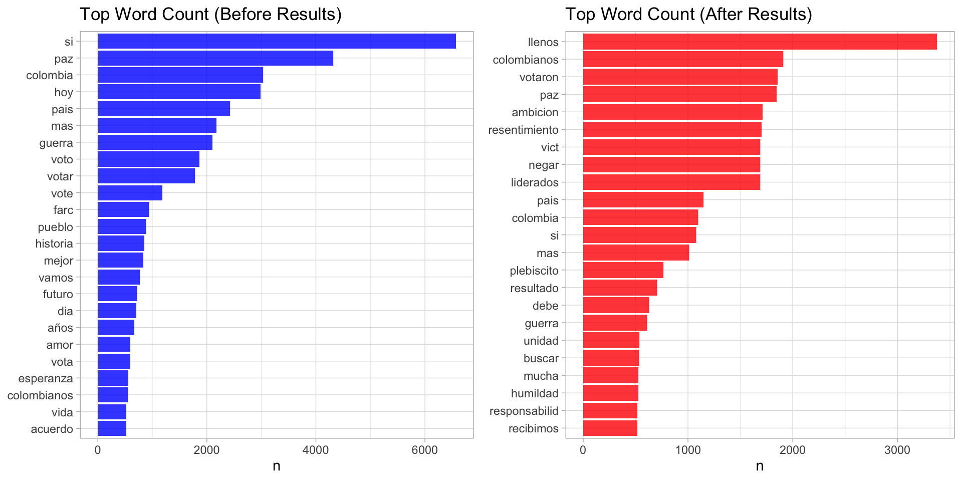
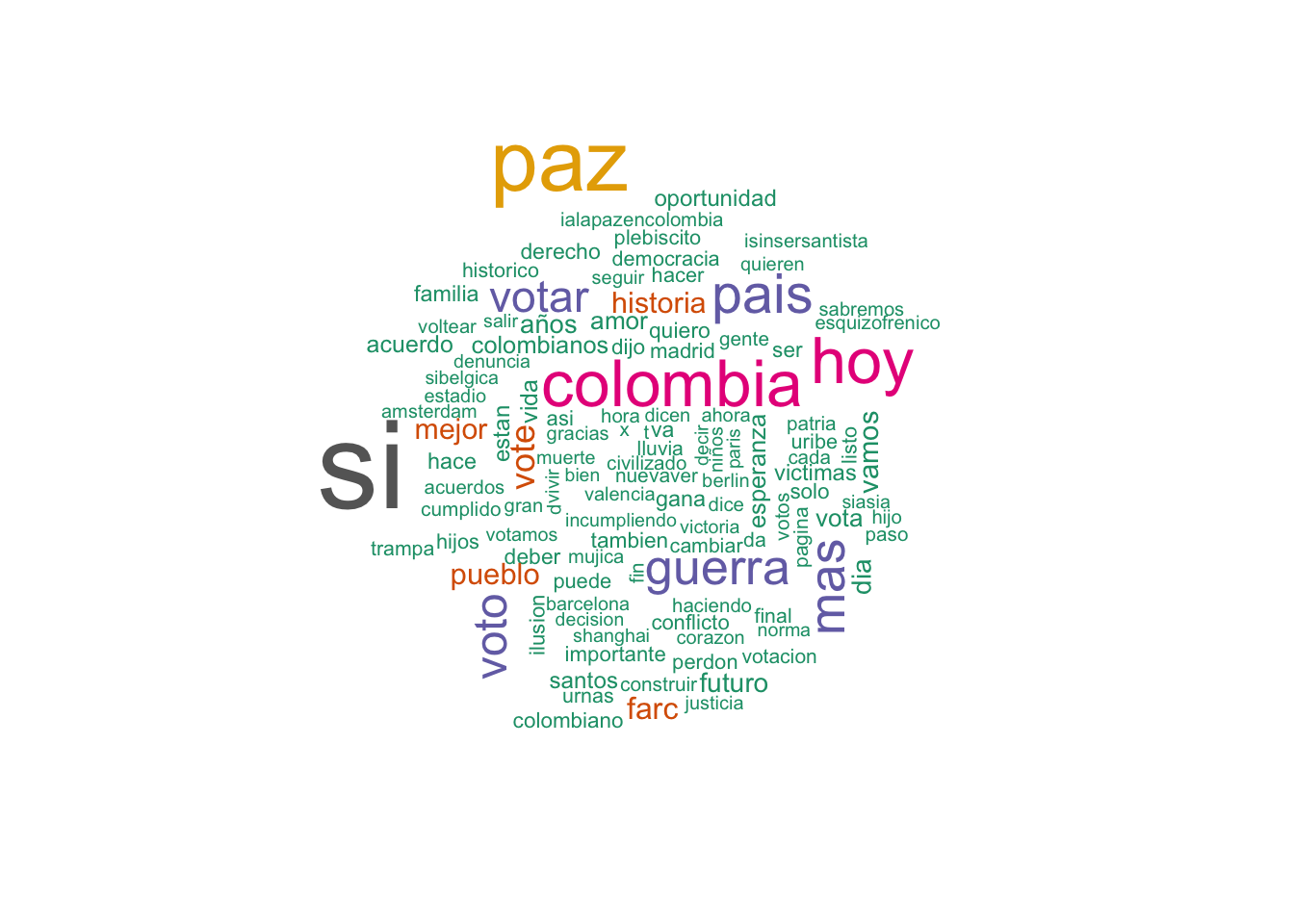
# Before the results.
wc.m <- wordcloud(
  words = word.count.m$word,
  freq = word.count.m$n,
  min.freq = 200,
  colors=brewer.pal(8, 'Dark2')
)
# After the results.
wordcloud(
  words = word.count.p$word,
  freq = word.count.p$n,
  min.freq = 100,
  colors=brewer.pal(8, 'Dark2')
)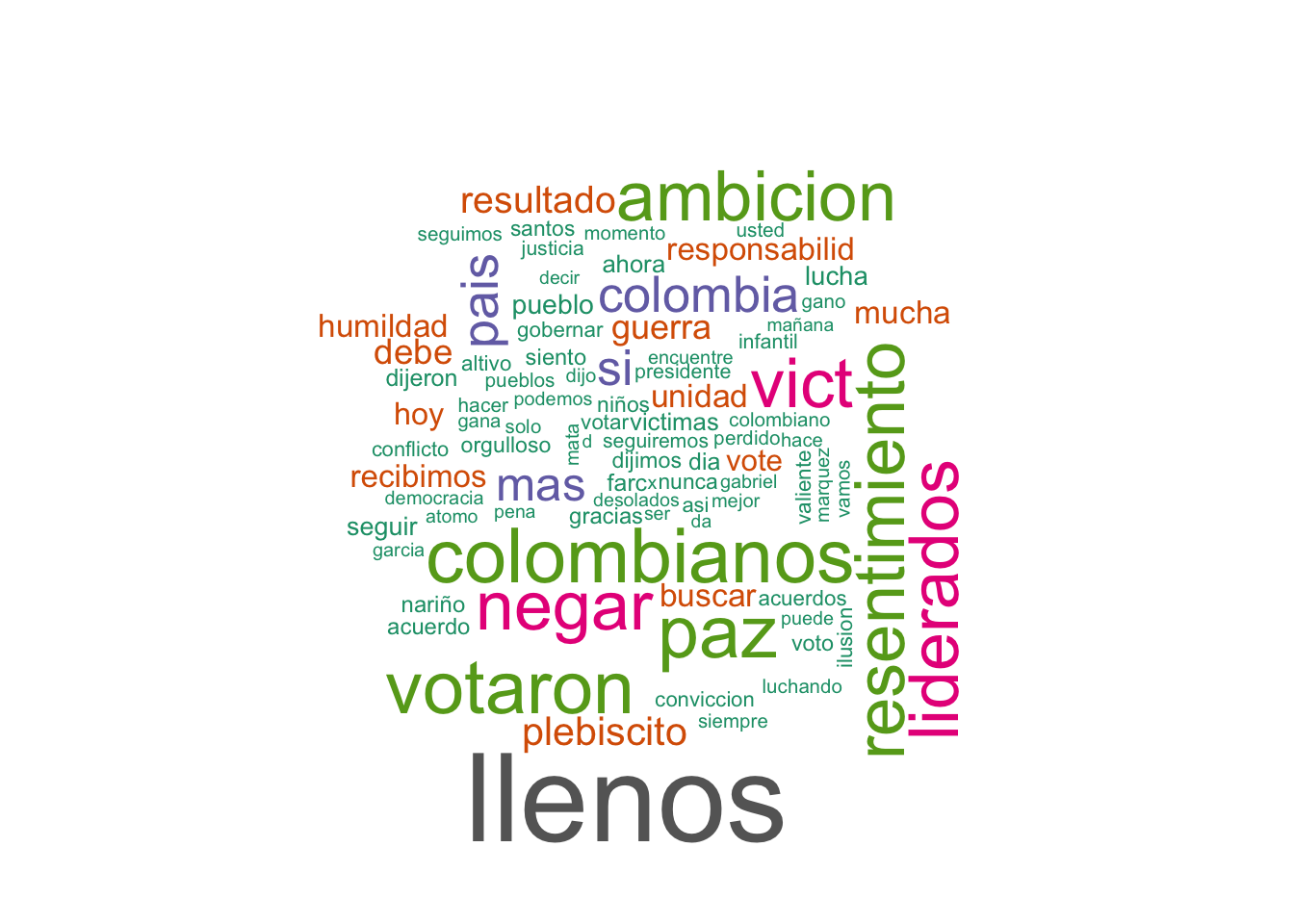
We can indeed see how the wording changes in these two time frames.
6.2 Hashtags
We can run an analogous analysis for hastags.
hashtags.unnested.df <- tweets.df %>%
  select(Created_At_Round, Hashtags) %>%
  unnest_tokens(input = Hashtags, output = hashtag)

hashtags.unnested.count <- hashtags.unnested.df %>%
  count(hashtag) %>%
  drop_na()
We plot the correspondinng word cloud.
wordcloud(
  words = str_c('#',hashtags.unnested.count$hashtag),
  freq = hashtags.unnested.count$n,
  min.freq = 40,
  colors=brewer.pal(8, 'Dark2')
)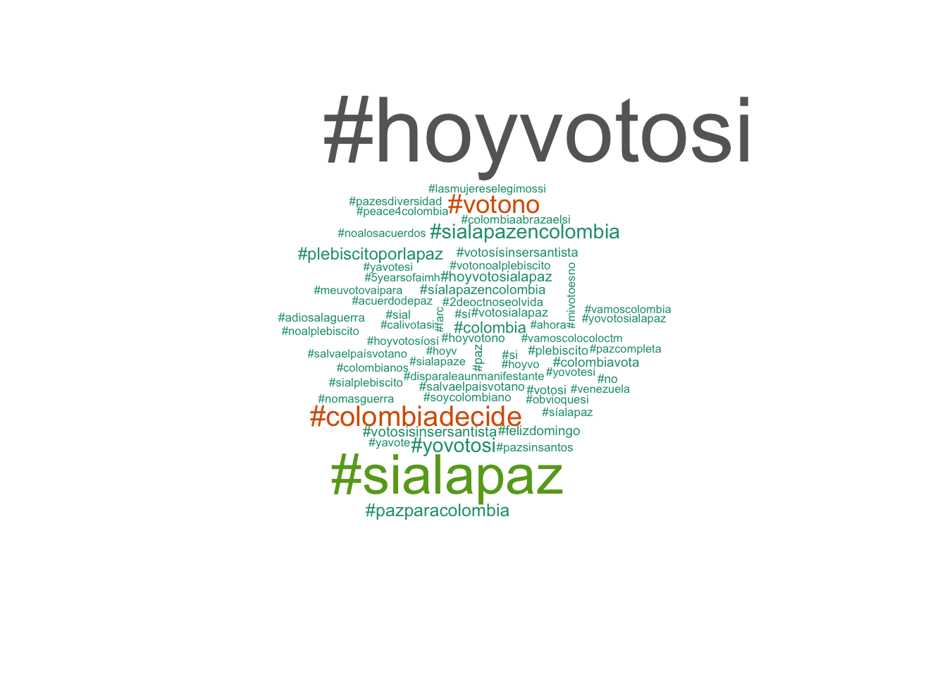
The most popular hashtag for the ‘YES’ and ‘NO’ are #hoyvotosi #notono respectively. Let us see the volume development of these hastags.
plt <- hashtags.unnested.df %>%
  filter(hashtag %in% c('hoyvotosi', 'votono')) %>%
  count(Created_At_Round, hashtag) %>%
  ggplot(mapping = aes(x  = Created_At_Round, y = n, color = hashtag)) +
    theme_light() +
    xlab(label = 'Date') +
    ggtitle(label = 'Top Hastags Counts') +
    geom_line() +
    scale_color_manual(values = c('hoyvotosi' = 'green3', 'votono' = 'red'))

plt %>% ggplotly()
Overall, the tweets supporting the ‘YES’ had much more volume. But this was not reflected on the results.
Remark: Compare with a brief initial analysis on the hastag volume over time.
7. Network Analysis
In this section we are going to describe how to encode and visualize tex data as a weighted netwok (graph). The main idea is to count pairwise relative occurence of words.
7.1 Bigram Analysis
7.1.1 Network Definition
We want to count pairwise occurences of words which apperar together in the text, this is what is known as bigram count.
bi.gram.words <- tweets.df %>%
  unnest_tokens(
    input = Text,
    output = bigram,
    token = 'ngrams',
    n = 2
  ) %>%
  filter(! is.na(bigram))

bi.gram.words %>%
  select(bigram) %>%
  head(10)
## # A tibble: 10 x 1
## bigram
## <chr>
## 1 paris bogota
## 2 bogota empanadas
## 3 colombia diferente
## 4 voy acercando
## 5 acercando puesto
## 6 puesto votacion
## 7 votacion siento
## 8 siento mariposas
## 9 mariposas estomago
## 10 estomago sientoNext, we filter for stop words and remove white spaces.
bi.gram.words %<>%
  separate(col = bigram, into = c('word1', 'word2'), sep = ' ') %>%
  filter(! word1 %in% stopwords.df$word) %>%
  filter(! word2 %in% stopwords.df$word) %>%
  filter(! is.na(word1)) %>%
  filter(! is.na(word2))
Finally, we group and count by bigram.
bi.gram.count <- bi.gram.words %>%
  count(word1, word2, sort = TRUE) %>%
  # We rename the weight column so that the
  # associated network gets the weights (see below).
  rename(weight = n)

bi.gram.count %>% head()
## # A tibble: 6 x 3
## word1 word2 weight
## <chr> <chr> <int>
## 1 llenos resentimiento 1688
## 2 ambicion votaron 1686
## 3 colombianos llenos 1686
## 4 liderados llenos 1686
## 5 llenos ambicion 1686
## 6 negar vict 1686- Weight Distribution
Let us plot the distribution of the weight values:
bi.gram.count %>%
  ggplot(mapping = aes(x = weight)) +
    theme_light() +
    geom_histogram() +
    labs(title = "Bigram Weight Distribution")
## `stat_bin()` using `bins = 30`. Pick better value with `binwidth`.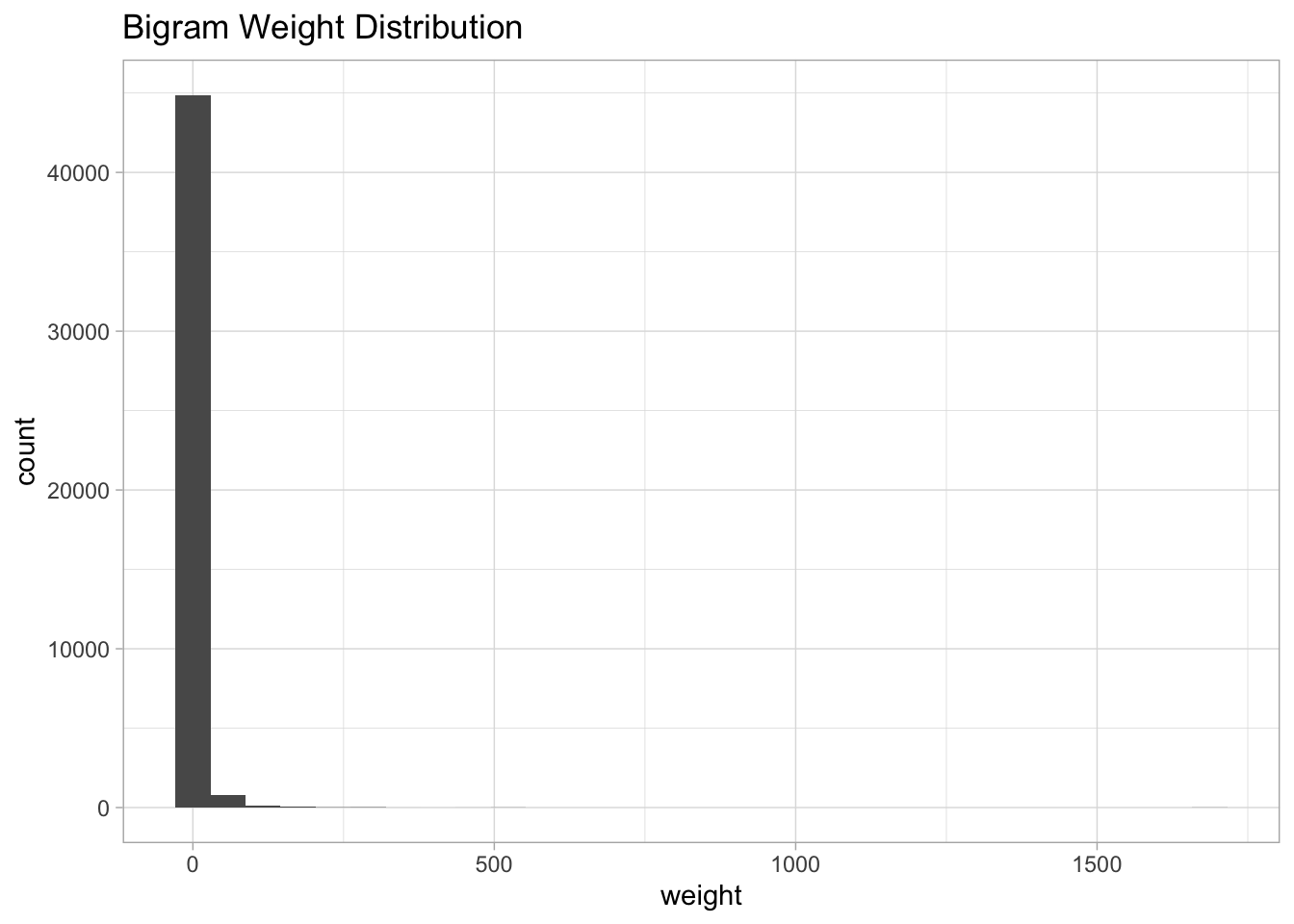
Note that is very skewed, for visualization purposes it might be a good idea to perform a transformation, e.g. log transform:
bi.gram.count %>%
  mutate(weight = log(weight + 1)) %>%
  ggplot(mapping = aes(x = weight)) +
    theme_light() +
    geom_histogram() +
    labs(title = "Bigram log-Weight Distribution")
## `stat_bin()` using `bins = 30`. Pick better value with `binwidth`.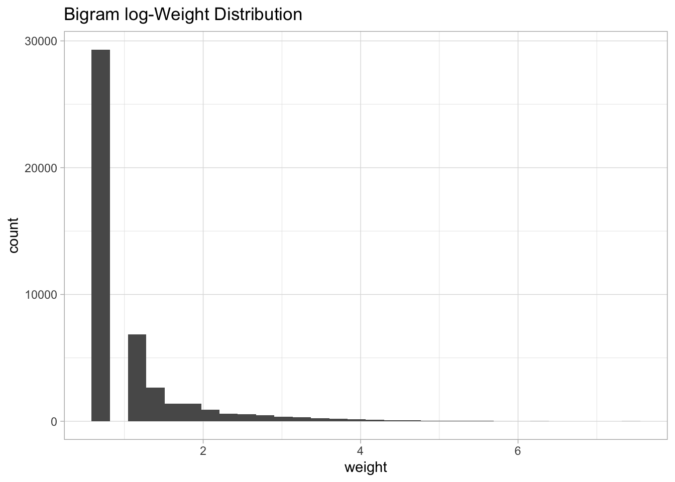
How to define a weighted network from a bigram count?
- Each word wis going to represent a node.
- Two words ae going to be connected if they appear as a bigram.
- The weight of an edge is the numer of times the bigram appears in the corpus.
- (Optional) We are free to decide if we want the graph to be directed or not.
We are going to use the igraph library to work with networks. The reference A User’s Guide to Network Analysis in R is highly recomended if you want to go deeper into network analysis in R.
For visualization purposes, we can set a threshold which defines the minimal weight allowed in the graph.
Remark: It is necessary to set the weight column name as weight (see igraph docs).
threshold <- 280

# For visualization purposes we scale by a global factor.
ScaleWeight <- function(x, lambda) {
  x / lambda
}

network <-  bi.gram.count %>%
  filter(weight > threshold) %>%
  mutate(weight = ScaleWeight(x = weight, lambda = 2E3)) %>%
  graph_from_data_frame(directed = FALSE)
Let us see how the network object looks like:
network## IGRAPH 92929e9 UNW- 30 27 --
## + attr: name (v/c), weight (e/n)
## + edges from 92929e9 (vertex names):
## [1] llenos --resentimiento ambicion --votaron llenos --colombianos
## [4] llenos --liderados llenos --ambicion negar --vict
## [7] liderados--resentimiento negar --votaron resultado--plebiscito
## [10] debe --buscar debe --plebiscito unidad --pais
## [13] unidad --buscar humildad --mucha mucha --responsabilid
## [16] pais --recibimos humildad --recibimos vote --paz
## [19] vote --ilusion vote --ilusion votar --si
## [22] guerra --mas pais --paz deber --cumplido
## + ... omitted several edgesLet us verify we have a weighted network:
is.weighted(network)## [1] TRUE7.1.2 Visualization
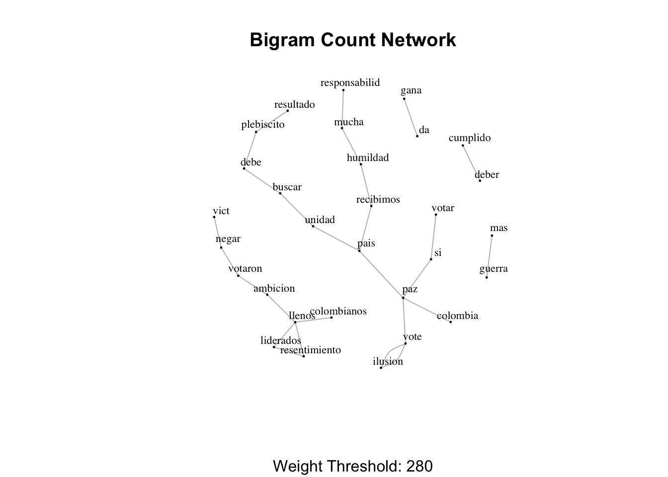
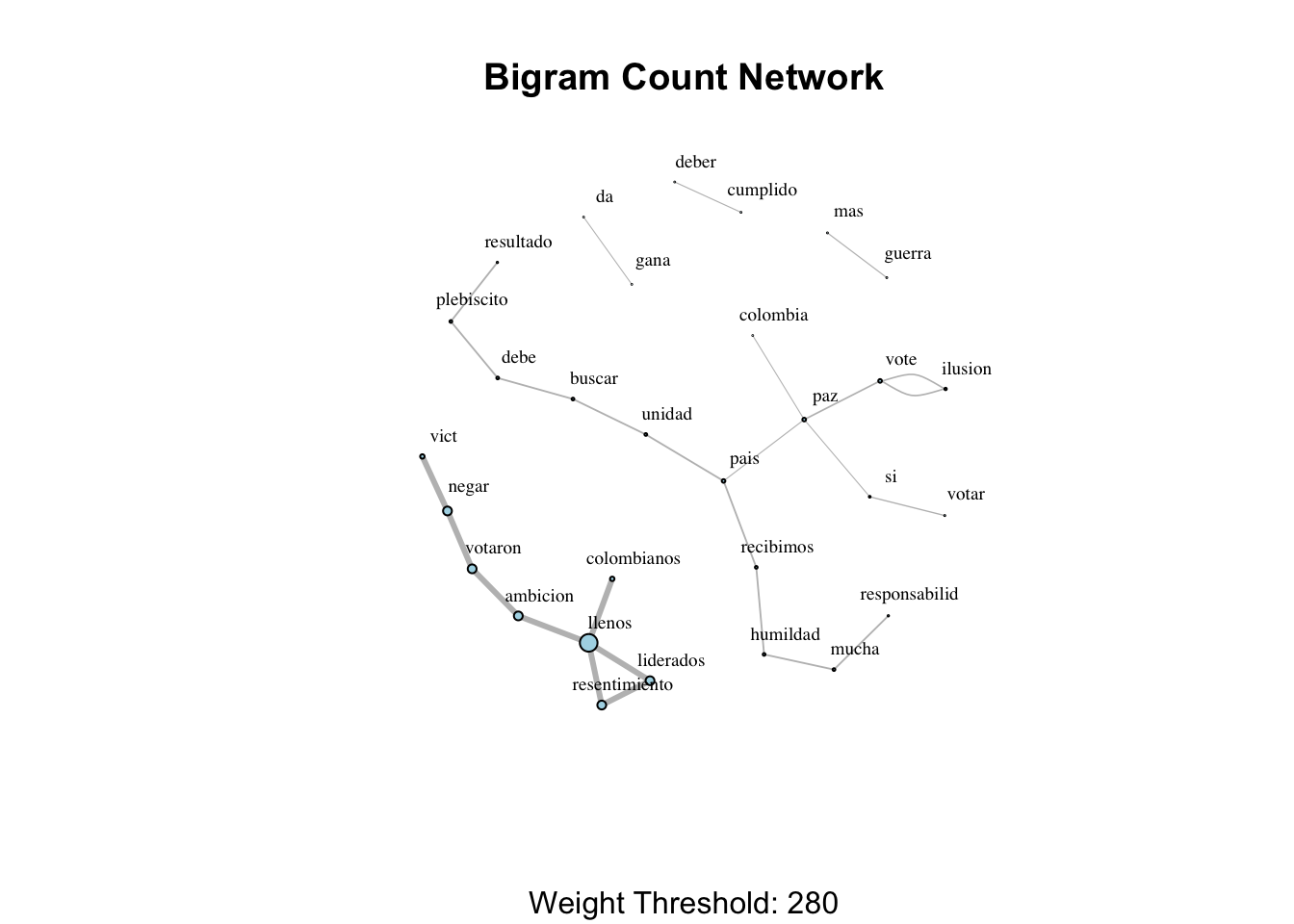
To visualize the network (here is a great reference for it) we can simply use the plot function with some additional parameters:
 plot(
  network,
  vertex.size = 1,
  vertex.label.color = 'black',
  vertex.label.cex = 0.7,
  vertex.label.dist = 1,
  edge.color = 'gray',
  main = 'Bigram Count Network',
  sub = glue('Weight Threshold: {threshold}'),
  alpha = 50
)
We can add some additional information to the visualization: Set the sizes of the nodes and the edges by the degree and weight respectively.
Remark: For a weighted network we can consider the weighted degree, which can be computed with the strength function.
# Store the degree.
V(network)$degree <- strength(graph = network)

# Compute the weight shares.
E(network)$width <- E(network)$weight/max(E(network)$weight)

plot(
  network,
  vertex.color = 'lightblue',
  # Scale node size by degree.
  vertex.size = 2*V(network)$degree,
  vertex.label.color = 'black',
  vertex.label.cex = 0.6,
  vertex.label.dist = 1.6,
  edge.color = 'gray',
  # Set edge width proportional to the weight relative value.
  edge.width = 3*E(network)$width ,
  main = 'Bigram Count Network',
  sub = glue('Weight Threshold: {threshold}'),
  alpha = 50
)
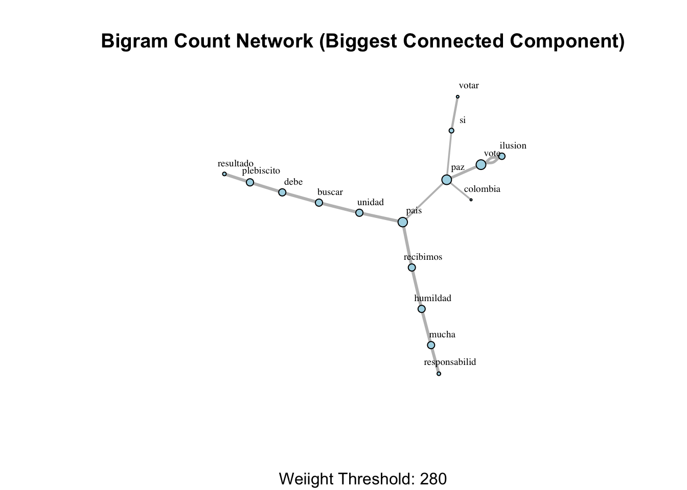
We can extract the biggest connected component of the network as follows:
# Get all connected components.
clusters(graph = network)
## $membership
## llenos ambicion colombianos liderados negar
## 1 1 1 1 1
## resentimiento votaron resultado debe plebiscito
## 1 1 2 2 2
## unidad buscar humildad mucha pais
## 2 2 2 2 2
## recibimos vote ilusion votar guerra
## 2 2 2 2 3
## deber si paz da vict
## 4 2 2 5 1
## responsabilid mas cumplido colombia gana
## 2 3 4 2 5
##
## $csize
## [1] 8 16 2 2 2
##
## $no
## [1] 5# Select biggest connected component.
V(network)$cluster <- clusters(graph = network)$membership
cc.network <- induced_subgraph(
graph = network,
vids = which(V(network)$cluster == which.max(clusters(graph = network)$csize))
)
cc.network ## IGRAPH e7f76e0 UNW- 16 16 --
## + attr: name (v/c), degree (v/n), cluster (v/n), weight (e/n), width
## | (e/n)
## + edges from e7f76e0 (vertex names):
## [1] resultado--plebiscito debe --buscar debe --plebiscito
## [4] unidad --pais unidad --buscar humildad --mucha
## [7] mucha --responsabilid pais --recibimos humildad --recibimos
## [10] vote --paz vote --ilusion vote --ilusion
## [13] votar --si pais --paz si --paz
## [16] paz --colombia# Store the degree.
V(cc.network)$degree <- strength(graph = cc.network)
# Compute the weight shares.
E(cc.network)$width <- E(cc.network)$weight/max(E(cc.network)$weight)
plot(
cc.network,
vertex.color = 'lightblue',
# Scale node size by degree.
vertex.size = 10*V(cc.network)$degree,
vertex.label.color = 'black',
vertex.label.cex = 0.6,
vertex.label.dist = 1.6,
edge.color = 'gray',
# Set edge width proportional to the weight relative value.
edge.width = 3*E(cc.network)$width ,
main = 'Bigram Count Network (Biggest Connected Component)',
sub = glue('Weiight Threshold: {threshold}'),
alpha = 50
)
We can go a steph further and make our visualization more dynamic using the networkD3 library.
# Treshold
threshold <- 250

network <-  bi.gram.count %>%
  filter(weight > threshold) %>%
  graph_from_data_frame(directed = FALSE)

# Store the degree.
V(network)$degree <- strength(graph = network)
# Compute the weight shares.
E(network)$width <- E(network)$weight/max(E(network)$weight)

# Create networkD3 object.
network.D3 <- igraph_to_networkD3(g = network)
# Define node size.
network.D3$nodes %<>% mutate(Degree = (1E-2)*V(network)$degree)
# Degine color group (I will explore this feature later).
network.D3$nodes %<>% mutate(Group = 1)
# Define edges width.
network.D3$links$Width <- 10*E(network)$width

forceNetwork(
  Links = network.D3$links,
  Nodes = network.D3$nodes,
  Source = 'source',
  Target = 'target',
  NodeID = 'name',
  Group = 'Group',
  opacity = 0.9,
  Value = 'Width',
  Nodesize = 'Degree',
  # We input a JavaScript function.
  linkWidth = JS("function(d) { return Math.sqrt(d.value); }"),
  fontSize = 12,
  zoom = TRUE,
  opacityNoHover = 1
)
Let us now decrease the threshold to get a more complex network (zoom out to see it all!).
# Treshold
threshold <- 80

network <-  bi.gram.count %>%
  filter(weight > threshold) %>%
  graph_from_data_frame(directed = FALSE)

# Store the degree.
V(network)$degree <- strength(graph = network)
# Compute the weight shares.
E(network)$width <- E(network)$weight/max(E(network)$weight)

# Create networkD3 object.
network.D3 <- igraph_to_networkD3(g = network)
# Define node size.
network.D3$nodes %<>% mutate(Degree = (1E-2)*V(network)$degree)
# Degine color group (I will explore this feature later).
network.D3$nodes %<>% mutate(Group = 1)
# Define edges width.
network.D3$links$Width <- 10*E(network)$width

forceNetwork(
  Links = network.D3$links,
  Nodes = network.D3$nodes,
  Source = 'source',
  Target = 'target',
  NodeID = 'name',
  Group = 'Group',
  opacity = 0.9,
  Value = 'Width',
  Nodesize = 'Degree',
  # We input a JavaScript function.
  linkWidth = JS("function(d) { return Math.sqrt(d.value); }"),
  fontSize = 12,
  zoom = TRUE,
  opacityNoHover = 1
)
7.2 Skipgram Analyis
7.2.1 Network Definition
Now we are going to consider skipgrams, which allow a “jump” in thw word count:
skip.window <- 2

skip.gram.words <- tweets.df %>%
  unnest_tokens(
    input = Text,
    output = skipgram,
    token = 'skip_ngrams',
    n = skip.window
  ) %>%
  filter(! is.na(skipgram))
For example, consider the tweet:
tweets.df %>%
  slice(4) %>%
  pull(Text)
## [1] " voy acercando puesto votacion siento mariposas estomago siento nervios felicidad "The skipgrams are:
skip.gram.words %>%
  select(skipgram) %>%
  slice(10:20)
## # A tibble: 11 x 1
## skipgram
## <chr>
## 1 voy
## 2 voy acercando
## 3 voy puesto
## 4 acercando
## 5 acercando puesto
## 6 acercando votacion
## 7 puesto
## 8 puesto votacion
## 9 puesto siento
## 10 votacion
## 11 votacion sientoWe now count the skipgrams containing two words.
skip.gram.words$num_words <- skip.gram.words$skipgram %>%
  map_int(.f = ~ ngram::wordcount(.x))

skip.gram.words %<>% filter(num_words == 2) %>% select(- num_words)

skip.gram.words %<>%
  separate(col = skipgram, into = c('word1', 'word2'), sep = ' ') %>%
  filter(! word1 %in% stopwords.df$word) %>%
  filter(! word2 %in% stopwords.df$word) %>%
  filter(! is.na(word1)) %>%
  filter(! is.na(word2))

skip.gram.count <- skip.gram.words  %>%
  count(word1, word2, sort = TRUE) %>%
  rename(weight = n)

skip.gram.count %>% head()
## # A tibble: 6 x 3
## word1 word2 weight
## <chr> <chr> <int>
## 1 llenos resentimiento 1688
## 2 colombianos llenos 1687
## 3 llenos votaron 1687
## 4 ambicion negar 1686
## 5 ambicion votaron 1686
## 6 colombianos resentimiento 16867.2.2 Visualization
Similarly as above, we construct and visualize the corresponding network (we select the biggest connected component):
# Treshold
threshold <- 80

network <-  skip.gram.count %>%
  filter(weight > threshold) %>%
  graph_from_data_frame(directed = FALSE)

# Select biggest connected component.
V(network)$cluster <- clusters(graph = network)$membership

cc.network <- induced_subgraph(
  graph = network,
  vids = which(V(network)$cluster == which.max(clusters(graph = network)$csize))
)

# Store the degree.
V(cc.network)$degree <- strength(graph = cc.network)
# Compute the weight shares.
E(cc.network)$width <- E(cc.network)$weight/max(E(cc.network)$weight)

# Create networkD3 object.
network.D3 <- igraph_to_networkD3(g = cc.network)
# Define node size.
network.D3$nodes %<>% mutate(Degree = (1E-2)*V(cc.network)$degree)
# Degine color group (I will explore this feature later).
network.D3$nodes %<>% mutate(Group = 1)
# Define edges width.
network.D3$links$Width <- 10*E(cc.network)$width

forceNetwork(
  Links = network.D3$links,
  Nodes = network.D3$nodes,
  Source = 'source',
  Target = 'target',
  NodeID = 'name',
  Group = 'Group',
  opacity = 0.9,
  Value = 'Width',
  Nodesize = 'Degree',
  # We input a JavaScript function.
  linkWidth = JS("function(d) { return Math.sqrt(d.value); }"),
  fontSize = 12,
  zoom = TRUE,
  opacityNoHover = 1
)
7.2.3 Node Importance
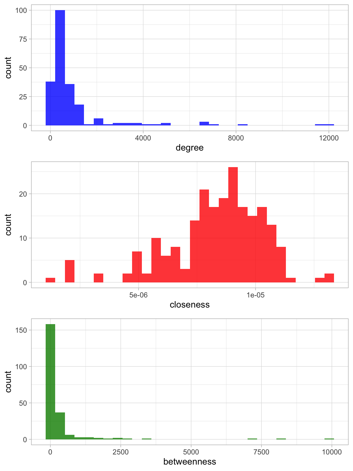
There are many notions of node importance in a network (A User’s Guide to Network Analysis in R, Section 7.2). Here we compare three of them
- Degree centrality
- Closeness centrality
- Betweenness centrality
# Compute the centrality measures for the biggest connected component from above.
node.impo.df <- tibble(
  word = V(cc.network)$name,
  degree = strength(graph = cc.network),
  closeness = closeness(graph = cc.network),
  betweenness = betweenness(graph = cc.network)
)
Now we rank the nodes with respect to these centrality measures:
- Degree centrality
node.impo.df %>%
  arrange(- degree) %>%
  head(10)
## # A tibble: 10 x 4
## word degree closeness betweenness
## <chr> <dbl> <dbl> <dbl>
## 1 si 12099 0.0000126 8305.
## 2 llenos 11806 0.00000225 0.5
## 3 paz 8210 0.0000132 9908.
## 4 votaron 6911 0.0000108 931.
## 5 resentimiento 6746 0.00000222 104.
## 6 ambicion 6744 0.00000223 110.
## 7 liderados 6744 0.00000125 0.5
## 8 negar 5058 0.00000222 1
## 9 mas 4919 0.0000110 2157.
## 10 pais 4718 0.0000109 2462- Closeness centrality
node.impo.df %>%
  arrange(- closeness) %>%
  head(10)
## # A tibble: 10 x 4
## word degree closeness betweenness
## <chr> <dbl> <dbl> <dbl>
## 1 paz 8210 0.0000132 9908.
## 2 hoy 3744 0.0000130 7284
## 3 si 12099 0.0000126 8305.
## 4 colombia 3804 0.0000115 3532.
## 5 voto 2898 0.0000112 2356.
## 6 vamos 772 0.0000111 528
## 7 guerra 2615 0.0000111 1326.
## 8 mas 4919 0.0000110 2157.
## 9 preferiria 163 0.0000110 0
## 10 injusta 333 0.0000110 274- Betweenness centrality
node.impo.df %>%
  arrange(- betweenness) %>%
  head(10)
## # A tibble: 10 x 4
## word degree closeness betweenness
## <chr> <dbl> <dbl> <dbl>
## 1 paz 8210 0.0000132 9908.
## 2 si 12099 0.0000126 8305.
## 3 hoy 3744 0.0000130 7284
## 4 colombia 3804 0.0000115 3532.
## 5 pueblo 3426 0.0000107 2767.
## 6 pais 4718 0.0000109 2462
## 7 voto 2898 0.0000112 2356.
## 8 mas 4919 0.0000110 2157.
## 9 colombiano 829 0.0000106 1821.
## 10 vote 3104 0.0000101 1718Let us see the distribution of these centrality measures.
plt.deg <- node.impo.df %>%
  ggplot(mapping = aes(x = degree)) +
    theme_light() +
    geom_histogram(fill = 'blue', alpha = 0.8, bins = 30)

plt.clo <- node.impo.df %>%
  ggplot(mapping = aes(x = closeness)) +
    theme_light() +
    geom_histogram(fill = 'red', alpha = 0.8, bins = 30)

plt.bet <- node.impo.df %>%
  ggplot(mapping = aes(x = betweenness)) +
    theme_light() +
    geom_histogram(fill = 'green4', alpha = 0.8, bins = 30)

plot_grid(
  ... = plt.deg,
  plt.clo,
  plt.bet,
  ncol = 1,
  align = 'v'
)
7.2.4 Community Detection
We can try to find clusters within the network. We use the Louvain Method for community detection:
comm.det.obj <- cluster_louvain(
  graph = cc.network,
  weights = E(cc.network)$weight
)

comm.det.obj
## IGRAPH clustering multi level, groups: 12, mod: 0.7
## + groups:
## $`1`
## [1] "vote" "ilusion" "colombia" "paz" "deber"
## [6] "dia" "niños" "nueva" "cumplido" "acuerdos"
## [11] "patria" "ponen" "dijeron" "farcsantos" "peligro"
## [16] "justicia" "estable" "construir" "gabriel" "garcia"
## [21] "proceso" "encuentre" "mata" "jaime" "sueño"
## [26] "viva" "social" "queremos" "infantil" "democracia"
## [31] "duradera" "marquez" "garzon" "solo" "t"
## [36] "pardo"
##
## + ... omitted several groups/verticesWe see that 12 groups where identified and the modularity is 0.7 (which is good, as it is close to 1).
Modularity is as chance-corrected statistic, and is defined as the fraction of ties that fall within the given groups minus the expected such fraction if the ties were distributed at random. (A User’s Guide to Network Analysis in R, Section 8.3.1)
Now we encode the membership as a node atribute (zoom and click on each node to explore the clusters).
V(cc.network)$membership <- membership(comm.det.obj)# We use the membership label to color the nodes.
network.D3$nodes$Group <- V(cc.network)$membership
forceNetwork(
Links = network.D3$links,
Nodes = network.D3$nodes,
Source = 'source',
Target = 'target',
NodeID = 'name',
Group = 'Group',
opacity = 0.9,
Value = 'Width',
Nodesize = 'Degree',
# We input a JavaScript function.
linkWidth = JS("function(d) { return Math.sqrt(d.value); }"),
fontSize = 12,
zoom = TRUE,
opacityNoHover = 1
)Let us collect the words per cluster:
membership.df <- tibble(
  word = V(cc.network) %>% names(),
  cluster = V(cc.network)$membership
)

V(cc.network)$membership %>%
  unique %>%
  sort %>%
  map_chr(.f = function(cluster.id) {

    membership.df %>%
      filter(cluster == cluster.id) %>%
      # Get 15 at most 15 words per cluster.
      slice(1:15) %>%
      pull(word) %>%
      str_c(collapse = ', ')

  })
## [1] "vote, ilusion, colombia, paz, deber, dia, niños, nueva, cumplido, acuerdos, patria, ponen, dijeron, farcsantos, peligro"
## [2] "pueblo, civilizado, dijo, esquizofrenico, listo, mujica, voltear, siento, valiente, lucha, altivo, dijimos, gobernar, nariño, orgulloso"
## [3] "si, hoy, votar, voto, sabremos, madrid, derecho, amsterdam, berlin, barcelona, shanghai, sibelgica, valencia, va, vota"
## [4] "guerra, mas, acuerdo, amor, salida, ahora, cambiar, puede, importante, buen, gobierno, hacer, historia, mal, victimas"
## [5] "hacemos, acompañan, estan, gaviria, militantes, pacho, espiritu, tc"
## [6] "hijo, arrebato, intolerancia, leonardo, posada, reina"
## [7] "llenos, colombianos, ambicion, liderados, negar, resentimiento, votaron, vict"
## [8] "resultado, debe, buscar, plebiscito, unidad, humildad, mucha, pais, recibimos, mejor, mama, soño, seguir, luchando, conviccion"
## [9] "da, hace, denuncia, estadio, haciendo, incumpliendo, norma, santos, trampa, gana"
## [10] "años, enemigo, quede, claro, matado, verdadero"
## [11] "votamos, familia, ninguna, abuelo, asesinado, farc, perdon, secuestrado, sino, premio, pase"
## [12] "bandera, carmena, disimula, venezuela, vergonzoso"7.3 Correlation Analysis (Phi Coefficient)
7.3.1 Network Definition
The focus of the phi coefficient is how much more likely it is that either both word X and Y appear, or neither do, than that one appears without the other. (Text Mining with R, Section 4.2.2). You can read more about this correlation measure here.
cor.words <- words.df %>%
  group_by(word) %>%
  filter(n() > 10) %>%
  pairwise_cor(item = word, feature = ID)
7.3.1 Visualization
Let us visualize the correlation of two important nodes in the network:
topic.words <- c('uribe', 'santos', 'farc')# Set correlation threshold.
threshold = 0.1
network <- cor.words %>%
rename(weight = correlation) %>%
# filter for relevant nodes.
filter((item1 %in% topic.words | item2 %in% topic.words)) %>%
filter(weight > threshold) %>%
graph_from_data_frame()
V(network)$degree <- strength(graph = network)
E(network)$width <- E(network)$weight/max(E(network)$weight)
network.D3 <- igraph_to_networkD3(g = network)
network.D3$nodes %<>% mutate(Degree = 5*V(network)$degree)
# Define color groups.
network.D3$nodes$Group <- network.D3$nodes$name %>%
as.character() %>%
map_dbl(.f = function(name) {
index <- which(name == topic.words)
ifelse(
test = length(index) > 0,
yes = index,
no = 0
)
}
)
network.D3$links %<>% mutate(Width = 10*E(network)$width)
forceNetwork(
Links = network.D3$links,
Nodes = network.D3$nodes,
Source = 'source',
Target = 'target',
NodeID = 'name',
Group = 'Group',
# We color the nodes using JavaScript code.
colourScale = JS('d3.scaleOrdinal().domain([0,1,2]).range(["gray", "blue", "red", "black"])'),
opacity = 0.8,
Value = 'Width',
Nodesize = 'Degree',
# We define edge properties using JavaScript code.
linkWidth = JS("function(d) { return Math.sqrt(d.value); }"),
linkDistance = JS("function(d) { return 550/(d.value + 1); }"),
fontSize = 18,
zoom = TRUE,
opacityNoHover = 1
)8. Conclusions & Remarks
In this post we explored how to get first insights from social media text data (Twitter). First, we presented how clean and normalize text data. Next, as a first approach, we saw how (pairwise) word counts give important information about the content and relations of the input text corpus. In addition, we studied how use networks as data structures to analyze and represent various count measures (bigram, skipgram, correlation). We also showed how we can cluster these words to get meaningful groups defining topics. But this is just the beginning! Next steps will include going into the meaning and class of the words (part of speech tagging and named entity recognition). We will explore these techniques in a future post.