This summer I had the great oportunity to attend an give a talk at Pydata Berlin 2018. The topic of my talk was On Laplacian Eigenmaps for Dimensionality Reduction. During the Unsupervised Learning & Visualization session Dr. Stefan Kühn presented a very interesting and visual talk on Manifold Learning and Dimensionality Reduction for Data Visualization and Feature Engineering and Dr. Evelyn Trautmann gave a nice application of spectral clustering (here are some nice notes around this subject) in the context of Extracting relevant Metrics. During our talks, spectral methods and the Graph Laplacian was the biggest intersection. This was an excelent oportunity to enhance the communication channels between pure math and its applications.
I want to acknowledge the organizers, volunteers and great speakers which made this conference possible.
Abstract
The aim of this talk is to describe a non-linear dimensionality reduction algorithm based on spectral techniques introduced in BN2003. The goal of non-linear dimensionality reduction algorithms, so called manifold learning algorithms, is to construct a representation of data on a low dimensional manifold embedded in a high dimensional space. The particular case we are going to present exploits various relations of geometric and spectral methods (discrete and continuous). Spectral methods are sometimes motivated by Marc Kac’s question Can One Hear the Shape of a Drum? which makes reference to the idea of recovering geometrical properties from the eigenvalues (spectrum) of a matrix (linear operator). Concretely, the approach followed in BN2003 has its foundation on the spectral analysis of the Graph Laplacian of the adjacency graph constructed from the data. The motivation of the construction relies on the continuous limit analogue, the Laplace-Beltrami operator, in providing an optimal embedding for manifolds. We will also indicate the relation with the associated heat kernel operator. Instead of following a pure formal approach we will present the main geometric and computational ideas of the algorithm. Hence, with basic knowledge of linear algebra (eigenvalues) and differential calculus you will be able to follow the talk. Finally we will show a concrete example in Python using scikit-learn.
Video
Slides
Here you can find the slides of the talk.
Suggestions and comments are always welcome!
Jupyter Notebook
In this notebook we present some simple examples which ilustrate the concepts discussed in the talk on Laplacian Eigenmaps for Dimensionality Reduction at PyData Berlin 2018.
The sample data, visualization code and object descriptions can be found in the documentation.
References:
1. Notebook Setup
import matplotlib.pyplot as plt
from mpl_toolkits.mplot3d import Axes3D
import numpy as np
from sklearn import manifold, datasets
from sklearn.utils import check_random_state
from sklearn.decomposition import PCA
2. Back to Our Toy Example
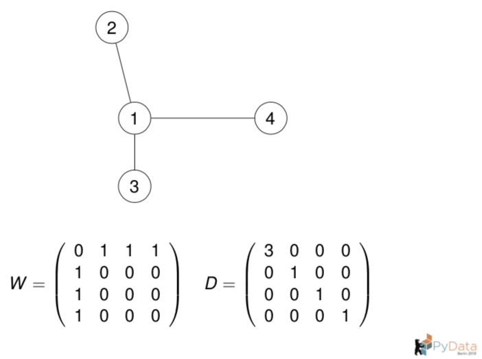
Let us compute the graph Laplacian from the adjacency matrix.
# Construct the adjacency matrix from the graph for n_neighbors = 1.
W = np.array([[0, 1, 1, 1],
              [1, 0, 0, 0],
              [1, 0, 0, 0],
              [1, 0, 0, 0]])

# Construct the degree matrix D from W.
D = np.diag(np.apply_along_axis(arr=W,
                                func1d=np.sum,
                                axis=0))
# Compute the graph Laplacian.
L = D - W

print(L)
[[ 3 -1 -1 -1]
[-1 1 0 0]
[-1 0 1 0]
[-1 0 0 1]]Let us use manifold.spectral_embedding to compute the projection onto \(\).
y = manifold.spectral_embedding(adjacency=W,
                                n_components=1,
                                norm_laplacian=False,
                                drop_first=True,
                                eigen_solver='lobpcg')

print(y)
[[ 0. ]
[-0.57735027]
[ 0.78867513]
[-0.21132487]]Let us verify the result. Recall that the first non zero eigenvalue of is \(_1 = 1\).
lambda_1 = 1

# Check if the previous output coincides with the analytical requirement.
np.array_equal(a1=np.dot(L, y),
a2=lambda_1*np.dot(D, y))TrueThus, \(y\) is a solution of \(Lf = _1 Df\) with \(_1 =1\).
3 Higher Dimensional Examples
3.1 S Curve
Reference: http://scikit-learn.org/stable/modules/generated/sklearn.datasets.make_s_curve.html
# Define the number of points to consider.
n_points = 3000

# Get the data and color map.
S_curve, S_colors = datasets.samples_generator.make_s_curve(n_points, random_state=0)

Axes3D

fig = plt.figure(figsize=(12, 12))
ax = fig.add_subplot(111, projection='3d')
ax.scatter(S_curve[:, 0], S_curve[:, 1], S_curve[:, 2],
           c=S_colors,
           cmap=plt.cm.Spectral)
ax.view_init(4, -72);
3.1.1 PCA
Let us see the result of PCA with n_components=2.
# Fit PCA object.
S_curve_pca = PCA(n_components=2).fit_transform(S_curve)

# Visualize the result.
fig = plt.figure(figsize=(12, 6))
ax = fig.add_subplot(111)
ax.scatter(S_curve_pca[:, 0], S_curve_pca[:, 1],
           c=S_colors,
           cmap=plt.cm.Spectral);
The result is coincides with ouur intuition, it is basically projecting to an axis so that the variance is maximized.
3.1.2 Spectral Embedding
Now let us use the method SpectralEmbedding from sklearn.
# Set the number of n_neighbors;
n_neighbors = 6

# Set the dimension of the target space.
n_components = 2

# Construct the SpectralEmbedding object.
se = manifold.SpectralEmbedding(n_components=n_components,
                                affinity= 'nearest_neighbors',
                                n_neighbors=n_neighbors)

# Fit the SpectralEmbedding object.
S_curve_red = se.fit_transform(X=S_curve)

# Visualize the result.
fig = plt.figure(figsize=(12, 6))
ax = fig.add_subplot(111)
ax.scatter(S_curve_red[:, 0], S_curve_red[:, 1],
           c=S_colors,
           cmap=plt.cm.Spectral);
We see that SpectralEmbedding unroll the S-curve so that the locallity is preserved on average.
Now let us consider n_neighbors >> 1.
# Set the number of n_neighbors;
n_neighbors = 1500

# Set the dimension of the target space.
n_components = 2

# Construct the SpectralEmbedding object.
se = manifold.SpectralEmbedding(n_components=n_components,
                                affinity= 'nearest_neighbors',
                                n_neighbors=n_neighbors)

# Fit the SpectralEmbedding object.
S_curve_red = se.fit_transform(X=S_curve)

# Visualize the result.
fig = plt.figure(figsize=(12, 6))
ax = fig.add_subplot(111)
ax.scatter(S_curve_red[:, 0], S_curve_red[:, 1],
           c=S_colors,
           cmap=plt.cm.Spectral);
The result is that the problem becomes more global. Thus, we get a similar result as PCA.
3.2 Two Dimensional Sphere \(S^2\)
Reference: http://scikit-learn.org/stable/auto_examples/manifold/plot_manifold_sphere.html
First we generate the data.
# Create our sphere.
n_samples = 5000

angle_parameter = 0.5 # Try 0.01
pole_hole_parameter = 8 # Try 50

random_state = check_random_state(0)
p = random_state.rand(n_samples) * (2 * np.pi - angle_parameter)
t = random_state.rand(n_samples) * np.pi

# Sever the poles from the sphere.
indices = ((t < (np.pi - (np.pi / pole_hole_parameter))) &
           (t > ((np.pi / pole_hole_parameter))))
colors = p[indices]
x, y, z = np.sin(t[indices]) * np.cos(p[indices]), \
          np.sin(t[indices]) * np.sin(p[indices]), \
          np.cos(t[indices])

sphere_data = np.array([x, y, z]).T
Let us visualize the data.
fig = plt.figure(figsize=(12, 12))
ax = fig.add_subplot(111, projection='3d')
ax.scatter(x, y, z,
           c=colors,
           cmap=plt.cm.Spectral);
3.2.1 PCA
Again, let us begin using PCA.
sphere_pca = PCA(n_components=2).fit_transform(sphere_data)

fig = plt.figure(figsize=(10, 10))
ax = fig.add_subplot(111)
ax.scatter(sphere_pca[:, 0], sphere_pca[:, 1],
           c=colors,
           cmap=plt.cm.Spectral);
3.3.2 Spectral Embedding
n_neighbors = 8
n_components = 2

# Fit the object.
se = manifold.SpectralEmbedding(n_components=n_components,
                                affinity='nearest_neighbors',
                                n_neighbors=n_neighbors)

sphere_data_red = se.fit_transform(X=sphere_data)
Let us visualize the results.
fig = plt.figure(figsize=(10, 10))
ax = fig.add_subplot(111)
ax.scatter(sphere_data_red[:, 0], sphere_data_red[:, 1],
           c=colors,
           cmap=plt.cm.Spectral);
We see how SpectralEmbedding unrolls the sphere.
Finally, let us take again n_neighbors >> 1.
n_neighbors = 1000

# Fit the object.
se = manifold.SpectralEmbedding(n_components=n_components,
                                affinity='nearest_neighbors',
                                n_neighbors=n_neighbors)

sphere_data_red = se.fit_transform(X=sphere_data)

fig = plt.figure(figsize=(10, 10))
ax = fig.add_subplot(111)
ax.scatter(sphere_data_red[:, 0], sphere_data_red[:, 1],
           c=colors,
           cmap=plt.cm.Spectral);