%%{init: {"theme": "white", "themeVariables": {"fontSize": "54px"}, "flowchart":{"htmlLabels": false}}}%%
flowchart TD
kernel["kernel"] --> spectral_sensity["Spectral Density"]
spectral_sensity --> polynomial["Polynomial Expansion"]
laplacian["Laplacian"] --> fourier["Fourier Transform"]
laplacian --> dirichlet["Dirichlet's BC"]
dirichlet --> spectral_decomposition["Spectral Decomposition"]
spectral_decomposition["Spectral Decomposition"] --> functional["Functional Calculus"]
polynomial --> identify_coefficients["Identify Coefficients"]
fourier --> identify_coefficients
functional --> identify_coefficients
identify_coefficients --> approximation["Approximation Formula"]
Introduction to Hilbert Spaces Approximations Gaussian Processes
A conceptual and practical viewpoint
Mathematician & Data Scientist
Outline
Reference Notebook 📓
Motivation: Some Applications
Gaussian Processes
Hilbert Space Approximation Deep Dive
Example: Birthdays Dataset
References
Motivation: Some Applications
Some Applications
Case Study: How popular is the President?
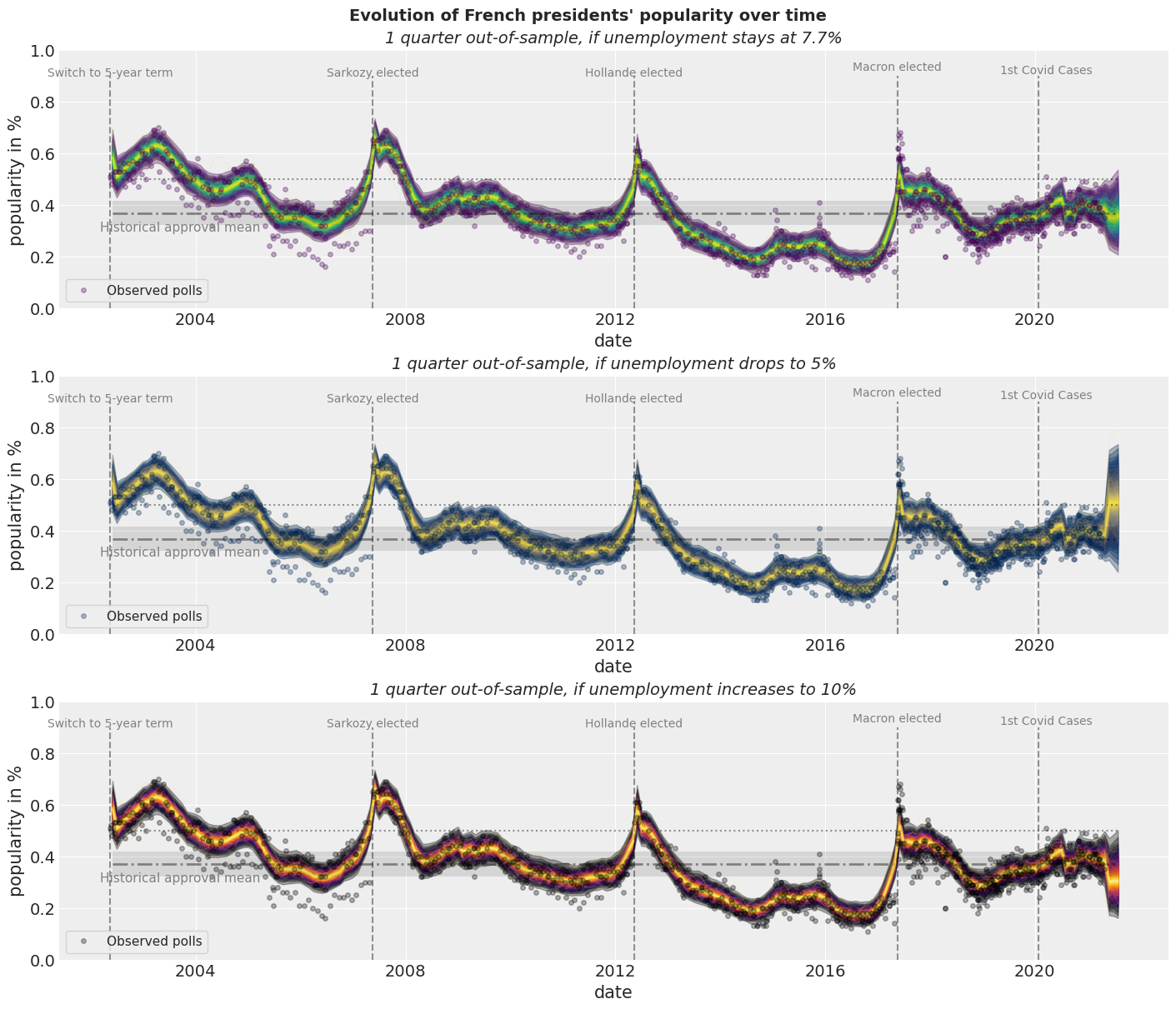
Some Applications
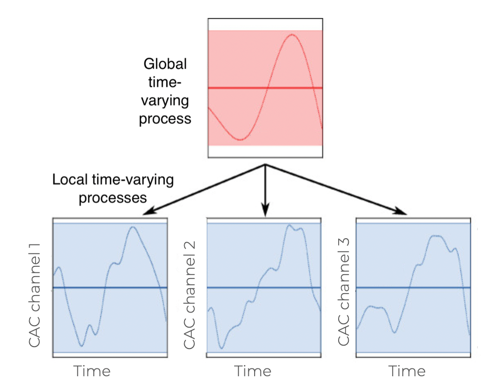
Time-Varying Regression Coefficients
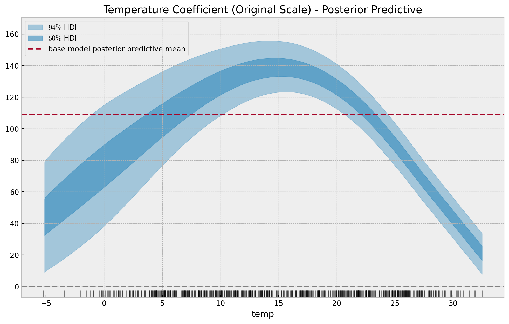
Some Applications
Changes in marketing effectiveness over time
Gaussian Processes
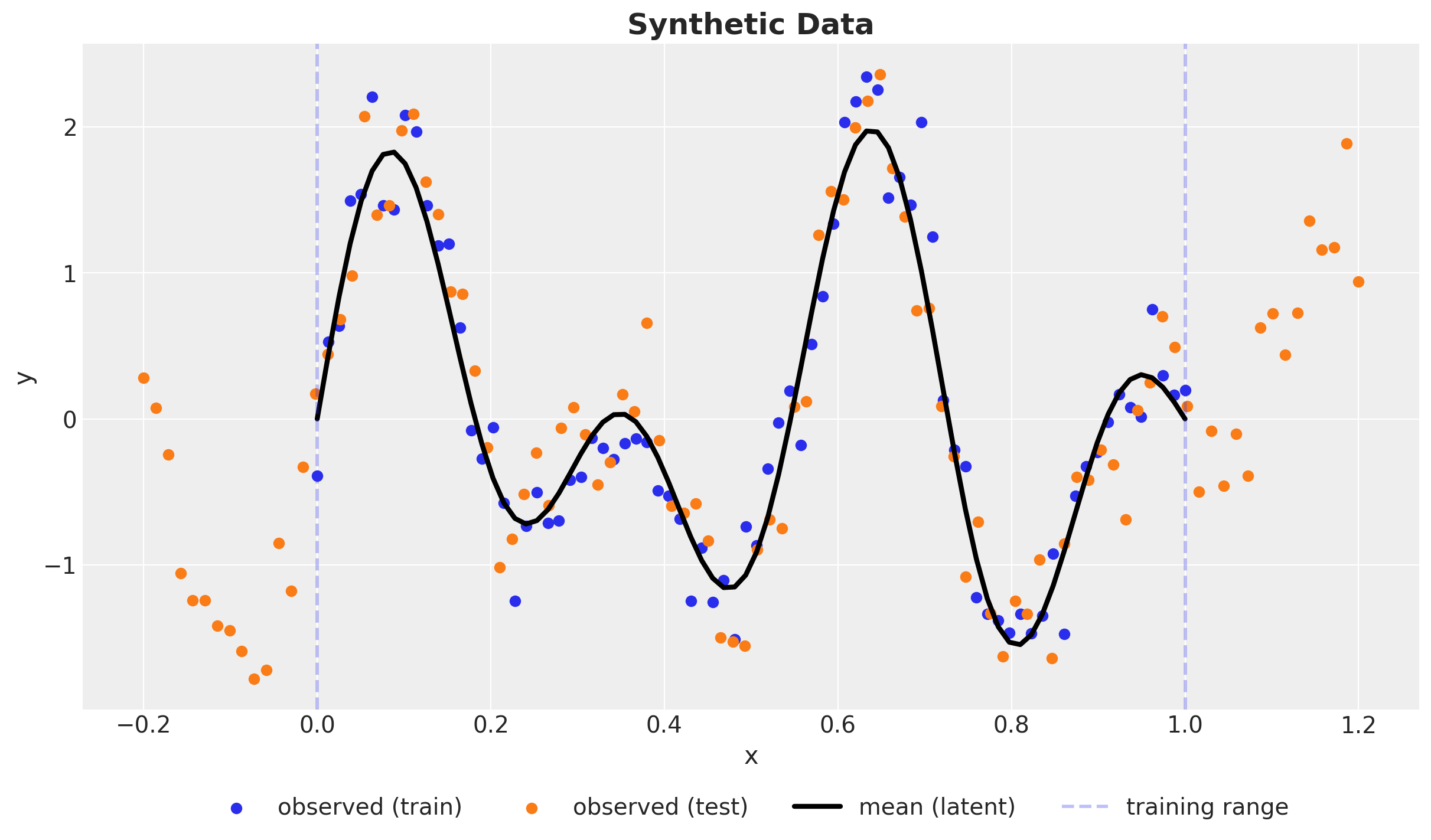
Synthetic Data
\(y \sim \text{Normal}(\sin(4 \pi x) + \sin(7 \pi x), 0.3^2)\)
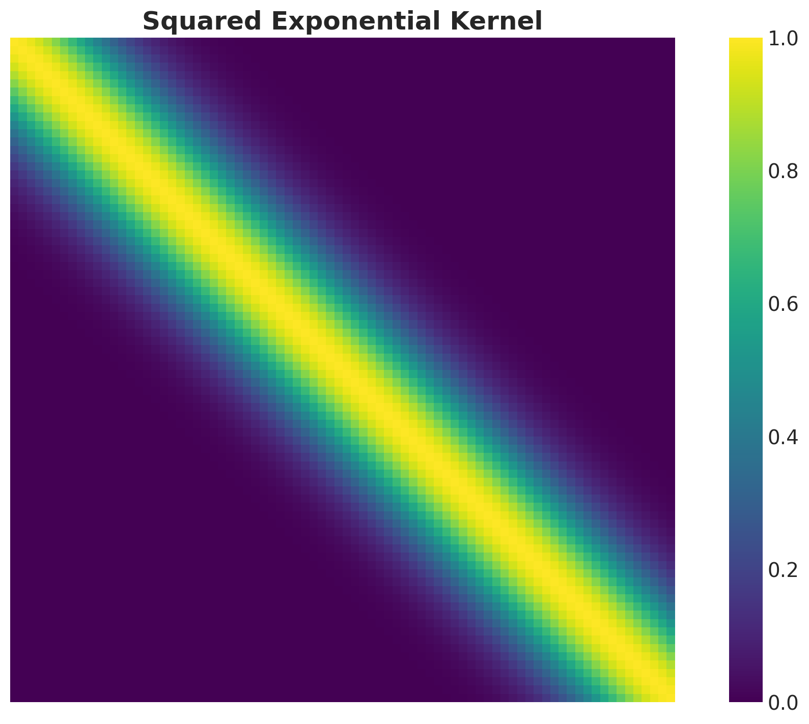
Kernel
A way to encode similarity between points
Example: Squared Exponential Kernel
\[ k(x, x') = a^ 2 \exp\left(-\frac{(x - x')^2}{2 \ell^2}\right) \]
Where \(a\) is the amplitude and \(\ell\) is the length-scale.
Note
Observe that the kernel just depends on the distance between points \(r = x - x'\). This is a property of stationary kernels.
Kernel Matrix
GP Model - Prior
Let us denote by \((x, y)\) and the training data and by \(x_{*}\) the test set for which we want to generate predictions. We define by \(f\) and \(f_*\) the latent functions for the training and test sets respectively.
\[ \left( \begin{array}{c} y \\ f_* \end{array} \right) \sim \text{MultivariateNormal}(0, \boldsymbol{K}) \]
where
\[ \boldsymbol{K} = \left( \begin{array}{cc} K(X, X) + \sigma^2_n I & K(X, X_*) \\ K(X_*, X) & K(X_*, X_*) \end{array} \right) \]
GP Model - Conditioning
\[ f_*|X, y, X_* \sim \text{MultivariateNormal}(\bar{f}_*, \text{cov}(f_*)) \]
where
\[ \begin{align*} \bar{f}_* &= K(X_*, X){\color{red}{(K(X, X) + \sigma^2_n I)^{-1}}} \\ \text{cov}(f_*) & = K(X_*, X_*) - K(X_*, X){\color{red}{(K(X, X) + \sigma^2_n I)^{-1}}} K(X, X_*) \end{align*} \]
Important
Taking the inverse of the kernel matrix is the most computationally expensive part of the GP model. It is of order \(\mathcal{O}(n^3)\).
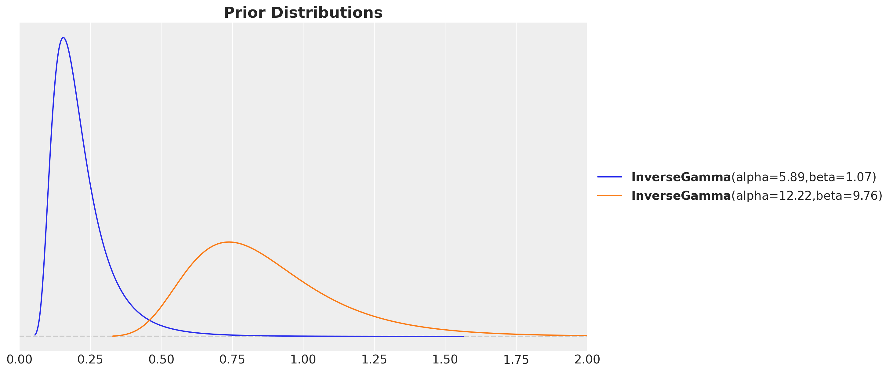
Kernel parameter priors
inverse_gamma_params_1 = pm.find_constrained_prior(
    distribution=pm.InverseGamma,
    lower=0.01,
    upper=0.4,
    init_guess={"alpha": 5, "beta": 3},
    mass=0.94,
)
inverse_gamma_params_2 = pm.find_constrained_prior(
    distribution=pm.InverseGamma,
    lower=0.5,
    upper=1.5,
    init_guess={"alpha": 5, "beta": 6},
    mass=0.94,
)

fig, ax = plt.subplots()
pz.InverseGamma(**inverse_gamma_params_1).plot_pdf(color="C0", ax=ax)
pz.InverseGamma(**inverse_gamma_params_2).plot_pdf(color="C1", ax=ax)
ax.set(xlim=(0, 2))
ax.set_title("Prior Distributions", fontsize=18, fontweight="bold");
Kernel parameter priors
GP Model in PyMC
with pm.Model() as gp_pymc_model:
    x_data = pm.MutableData("x_data", value=x_train)

    kernel_amplitude = pm.InverseGamma("kernel_amplitude", ...)
    kernel_length_scale = pm.InverseGamma("kernel_length_scale", ...)
    noise = pm.InverseGamma("noise", ...)

    mean = pm.gp.mean.Zero()
    cov = kernel_amplitude**2 * pm.gp.cov.ExpQuad(
        input_dim=1, ls=kernel_length_scale
    )
    gp = pm.gp.Latent(mean_func=mean, cov_func=cov)
    f = gp.prior("f", X=x_data[:, None])

    pm.Normal("likelihood", mu=f, sigma=noise, observed=y_train_obs)
GP Model in PyMC
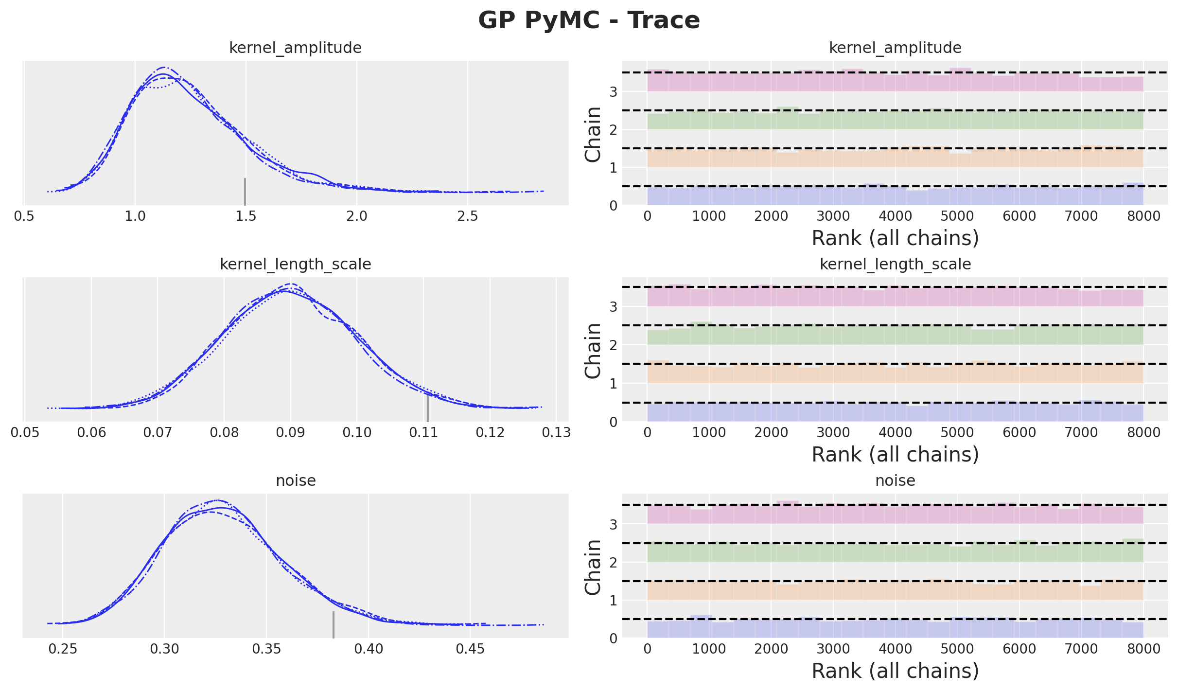
GP Model - Prior Predictions
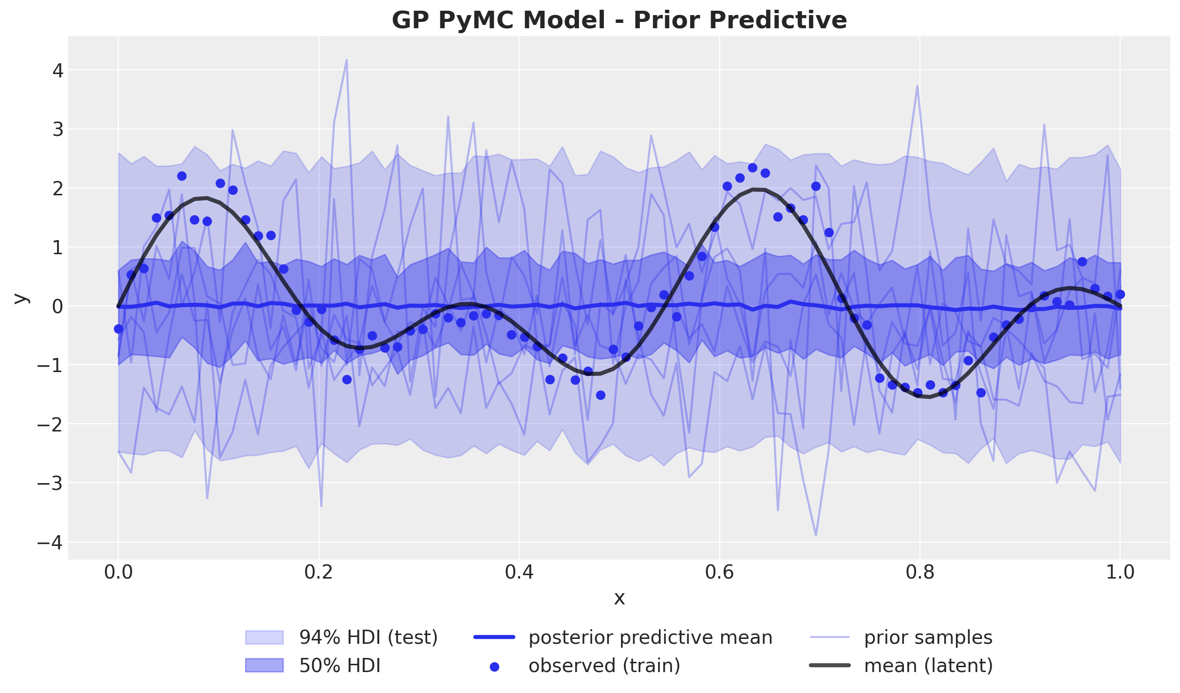
GP Model - Posterior Distributions
Out-of-Sample Predictions
conditional method
with gp_pymc_model:
    x_star_data = pm.MutableData("x_star_data", x_test)
    f_star = gp.conditional("f_star", x_star_data[:, None])
    pm.Normal("likelihood_test", mu=f_star, sigma=noise)

    gp_pymc_idata.extend(
        pm.sample_posterior_predictive(
            trace=gp_pymc_idata,
            var_names=["f_star", "likelihood_test"],
            random_seed=rng_subkey[1].item(),
        )
    )
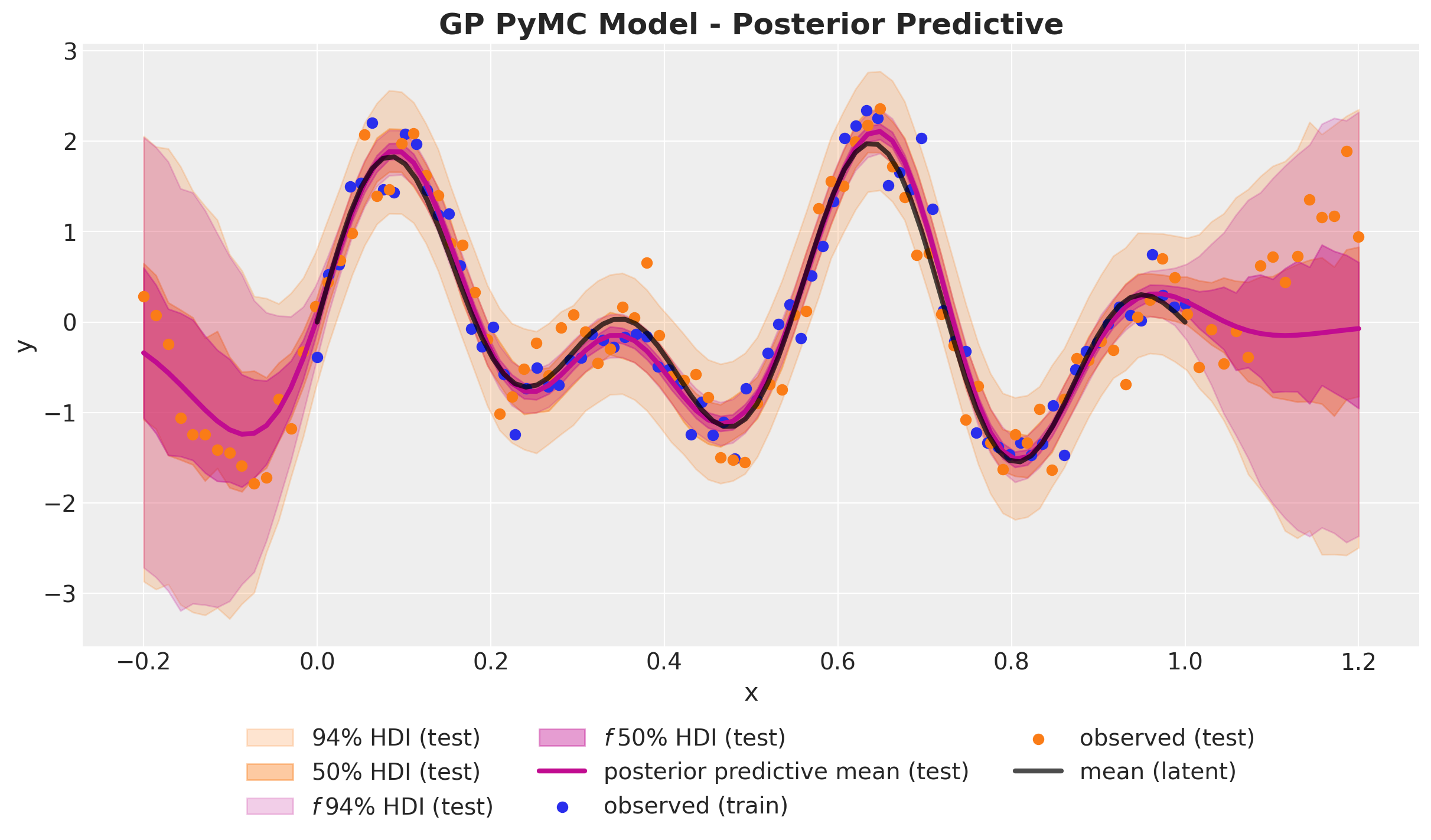
GP Model - Posterior Predictive
Hilbert Space Gaussian Process (HSGP) Approximation
HSGP Deep Dive
Approach Summary 🤓
Strategy: Approximate the Gram matrix \(K\) with a matrix \(\tilde{K}\) with a smaller rank \(m < n\).
Key Idea: Interpret the covariance function as the kernel of a pseudo-differential operator and approximate it using Hilbert space methods.
Result: A reduced-rank approximation for the covariance function, where the basis functions are independent of the covariance functions and their parameters (plus asymptotic convergence).
Hilbert Space Approximation
Hilbert Space Approximation
Approximation Strategy Steps
- D-Tour: Eigenvalues and Eigenvectors
- We recall the spectral density \(S(\omega)\) associated with a stationary kernel function \(k\).
- We approximate the spectral density \(S(\omega)\) as a polynomial series in \(||\omega||^2\).
- We can interpret these polynomial terms as powers of the Laplacian operator. The key observation is that the Fourier transform of the Laplacian operator is \(||\omega||^2\).
- Next, we impose Dirichlet boundary conditions on the Laplacian operator which makes it self-adjoint and with a discrete spectrum.
- We identify the expansion in (2) with the sum of powers of the Laplacian operator in the eigenbasis of (4).
- We arrive at the final approximation formula and explicitly compute the terms for the squared exponential kernel in the one-dimensional case.
Eigenvalues and Eigenvectors
Recall that given a matrix \(A\) (or a linear operator) the eigenvalues and eigenvectors are the solutions to the equation
\[A v = \lambda v\]
where \(v \neq \vec{0}\) is the eigenvector and \(\lambda\) is the eigenvalue.
The spectrum of a matrix is the set of its eigenvalues.
Example - \(2 \times 2\) Matrix
\[ A = \begin{pmatrix} 1 & 2 \\ 2 & 1 \end{pmatrix} \]
The eigenvalues are \(\lambda_1 = 3\) and \(\lambda_2 = -1\) with eigenvectors:
\[ v_1 = \frac{1}{\sqrt{2}} \begin{pmatrix} 1 \\ 1 \end{pmatrix} \quad \text{and} \quad v_2 = \frac{1}{\sqrt{2}} \begin{pmatrix} -1 \\ 1 \end{pmatrix} \]
Properties
\[ v_1^{T} v_2 = 0 \quad \text{and} \quad v_1^{T} v_1 = v_2^{T} v_2 = 1 \]
The Spectral Theorem
The spectral theorem states that we can always find such orthonormal basis of eigenvectors for a symmetric matrix.
Observe that if we consider the change-of-basis matrix
\[ Q = \begin{pmatrix} v_1 & v_2 \end{pmatrix} \]
then we can write the matrix \(A\) in the new basis as
\[ D = Q^{T} A Q = \begin{pmatrix} 3 & 0 \\ 0 & -1 \end{pmatrix} \]
Code Example
import jax.numpy as jnp

A = jnp.array([[1.0, 2.0], [2.0, 1.0]])

# Compute eigenvalues and eigenvectors
eigenvalues, eigenvectors = jnp.linalg.eig(A)

print(f"Eigenvalues: {eigenvalues}\nEigenvectors:\n{eigenvectors}")

>> Eigenvalues: [ 3.+0.j -1.+0.j]
>> Eigenvectors:
>> [[ 0.70710678+0.j -0.70710678+0.j]
>> [ 0.70710678+0.j  0.70710678+0.j]]


# Change of basis matrix
Q = eigenvectors
Q.T @ A @ Q

>> Array([[ 3.00000000e+00+0.j,  4.44089210e-16+0.j],
[ 6.10622664e-16+0.j, -1.00000000e+00+0.j]], dtype=complex128)Spectral Projections
Another important consequence of the spectral theorem is that we can decompose the matrix \(A\) as a sum of projections onto its eigenspaces. That is, we can write re-write \(A\) as
\[ A = \sum_{j=1}^{2} \lambda_i v_j v_j^{T} \]
Projections
Observe that the operator \(P_{j} = v_j v_j ^{T}\) is indeed a projection operator, that is \(P^2 = P\) and \(P^T = P\), since the \(v_j\) constitutes an orthonormal basis.
Code Example
def proj(v, x):
    return jnp.dot(v, x) * v

def matrix_proj(x):
    return eigenvalues[0] * proj(Q[:, 0], x) + eigenvalues[1] * proj(Q[:, 1], x)

# First eigenvector
matrix_proj(Q[:, 0])  / eigenvalues[0]
>> Array([0.70710678+0.j, 0.70710678+0.j], dtype=complex128)

# Second eigenvector
matrix_proj(Q[:, 1])  / eigenvalues[1]
>> Array([-0.70710678-0.j,  0.70710678-0.j], dtype=complex128)

# Arbitrary vector
v = jnp.array([1.0, 2.0])
jnp.allclose(jnp.dot(A, v), matrix_proj(v))
>> Array(True, dtype=bool)
Functional Calculus
The functional calculus is a generalization of the Taylor series for functions to operators. Given a function \(f\) we can define the operator \(f(A)\) as
\[ f(A) = \sum_{j=1}^{2} \color{red}{f(\lambda_j)} \color{blue}{v_j v_j^{T}} \]
Examples
- \(f(z) = z\) we recover the operator \(A\).
- \(f(z) = 1\) we get the identity operator \(I\).
- \(f(z) = z^2\) we get the operator \(A^2\).
- \(f(z) =e^{z}\) we get the operator \(\exp(A)\).
Example: Exponential of a Matrix
Consider the exponential of the matrix \(A\) defined as
\[ \exp(A) = \sum_{j=0}^{\infty} \frac{A^j}{j!} \]
Example: Exponential of a Matrix
On the other hand, we can use the fact that \(A = Q D Q^{T}\) and that \(Q\) is an orthogonal matrix to write
\[ \exp(A) = \sum_{j=0}^{\infty} \frac{(Q D Q^{T})^j}{j!} = Q \left(\sum_{j=0}^{\infty} \frac{D^j}{j!}\right) Q^{T} = Q \exp(D) Q^{T} \]
and observe that \(\exp(D)\) is a diagonal matrix with the exponential of the diagonal elements:
Spectral Densities
In the case a kernel function is stationary, we can use the spectral representation of the kernel function (Bochner’s theorem):
\[ k(r) = \frac{1}{(2 \pi)^{d}}\int_{\mathbb{R}^{d}} e^{i \omega^{T} r} d\mu(\omega) \]
where \(\mu\) is a positive measure. If this measure has a density, it is called the spectral density \(S(\omega)\) corresponding to the covariance function, i.e. \(d\mu(\omega) = S(\omega) d\omega\).
Spectral Density - Example
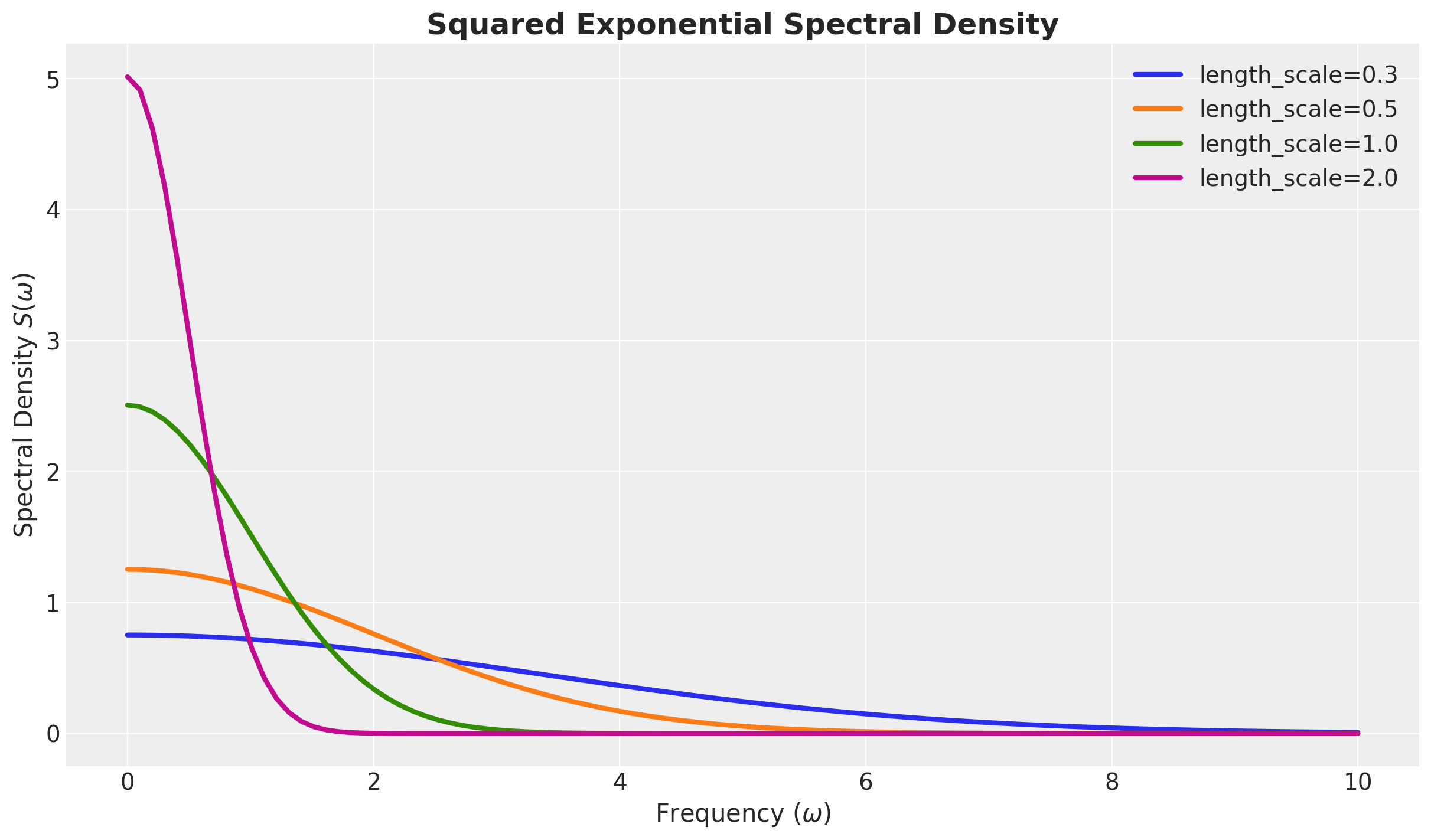
For the squared exponential kernel, it can be shown that
\[ S(\omega) = a^2(2 \pi \ell^2)^{d/2} \exp\left(-2\pi^2\ell^2\omega^2\right) \]
For the special case \(d=1\) we have
\[ S(\omega) = a^2 \sqrt{2 \pi} \ell \exp\left(-2\pi^2\ell^2\omega^2\right) \]
Tip
Note the similarity between the spectral density and the Fourier transform. For Gaussian-like kernels, like the squared exponential, we expect the associated spectral density to also be Gaussian-like.
\(S(\omega)\) Squared Exponential
Formal Power Expansion of the Spectral Density
Let us assume the kernel function is isotropic, i.e. it just depends on the Euclidean norm \(||r||\).
\(S(\omega)\) is also isotropic.
Write \(S(||\omega||) = \psi(||\omega||^2)\) for a suitable function \(\psi\).
We can expand \(\psi\) (Taylor-like expansion)
\[ \begin{align*} \psi(||\omega||^2) = a_0 + a_1 (||\omega||^2) + a_2 (||\omega||^2)^2 + a_3 (||\omega||^2)^3 + \cdots \end{align*} \]
The Laplace Operator
Recall the Laplace operator is defined as
\[ - \nabla^2 f = \sum_{i=1}^{d} \frac{\partial^2 f}{\partial x_i^2} \]
Tip
The Laplacian has many good properties:
Positive semi-definite
Elliptic
Self-adjoint (appropriate boundary conditions)
Kernel as a function of \(\nabla^2\)
One can verify that the Fourier transform of the Laplacian is
\[ \mathcal{F}[\nabla^2 f](\omega) = - ||\omega||^2 \mathcal{F}[f] \]
We can write the integral operator associated with the kernel
\[ \mathcal{K} := \int_{\mathbb{R}^d} k(\cdot, x')\phi(x') dx' \]
as
\[ \mathcal{K} = a_0 + a_1 (- \nabla^2) + a_2 (-\nabla^2)^2 - a_3 (-\nabla^2)^3 + \cdots \]
Dirichlet’s Laplacian
Boundary Conditions?
The most common boundary conditions are the Dirichlet boundary conditions, which are defined by requiring that the function vanishes on the boundary of the domain.
\[ \begin{align*} -\nabla^2 f &= \lambda f \quad \text{in} \quad \Omega \\ f &= 0 \quad \text{on} \quad \partial \Omega \end{align*} \]
Dirichlet’s Laplacian - Spectrum
It is is a self-adjoint operator defined on the Hilbert space \(L^{2}(\Omega)\) equipped with the Lebesgue measure. That is,
\[ \int_{\Omega} (-\nabla^2 f(x)) g(x) dx = \int_{\Omega} f(x) (-\nabla^2 g(x)) dx \]
It has discrete spectrum with eigenvalues \(\lambda_j \rightarrow \infty\) and eigenfunctions \(\phi_j\) that form an orthonormal basis of \(L^2(\Omega)\), so that \[ \int_{\Omega} \phi_{j}(x) \phi_{k}(x) dx = \delta_{jk} \]
Example - One Dimensional Box
\(\Omega = [-L, L] \subset \mathbb{R}\)
\[ \frac{d^2 \phi}{dx^2} = - \lambda \phi \quad \text{with} \quad \phi(-L) = \phi(L) = 0 \]
Spectrum?
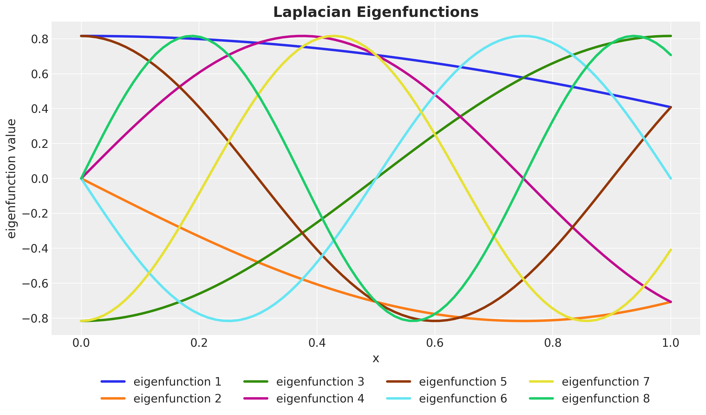
\[ \phi_j(x) = \sqrt{\frac{1}{L}} \sin\left(\frac{\pi j (x + L)}{2L}\right) \quad \text{and} \quad \lambda_j = \left(\frac{j \pi}{2L}\right)^2 \]
for \(j = 1, 2, \ldots\).
HSGP: Functional Calculus
\[ -\nabla^2 f(x) = \int_{\Omega} \overbrace{\left[\sum_{j} \lambda_{j} \phi_{j}(x) \phi_{j}(x')\right]}^{l(x, x')} f(x') dx' \]
We can construct powers of \(-\nabla^2\) as
\[ (- \nabla^2)^{s} f(x) = \int_{\Omega} {\color{red}{\overbrace{\left[\sum_{j} \lambda_{j}^{s} \phi_{j}(x) \phi_{j}(x')\right]}^{l^s(x, x')}}} f(x') dx'. \]
HSGP: Coefficients Identification
Use the formal expansion of \(\mathcal{K}\) in terms of powers of \(\nabla^2\):
\[ \begin{align*} & \left[ a_{0} + a_{1}(-\nabla^2) + a_{2}(-\nabla^2)^2 + \cdots \right]f(x) = \\ &\int_{\Omega} \left[a_{0} + a_{1} l(x, x') + a_{2} l^{2}(x, x') + \cdots \right] f(x') dx' \end{align*} \]
This implies we can approximate the kernel as
\[ \begin{align*} k(x, x') \approx & \: a_{0} + a_{1} l(x, x') + a_{2} l^{2}(x, x') + \cdots \\ \approx & \sum_{j} {\color{red}{\underbrace{\left[ a_{0} + a_{1} \lambda_{j} + a_{2} \lambda_{j}^2 + \cdots \right]}_{S(\sqrt{\lambda_{j}})}}} \phi_{j}(x) \phi_{j}(x') \end{align*} \]
HSGP: Final Formula
In summary, we have the following approximation formula for the kernel function:
\[ \boxed{ k(x, x') \approx \sum_{j}^{m} \color{red}{S(\sqrt{\lambda_j})}\color{blue}{\phi_{j}(x) \phi_{j}(x')} } \]
That is, the model of the Gaussian process \(f\) can be written as
\[ f(x) \sim \text{MultivariateNormal}(\boldsymbol{\mu}, \Phi\mathcal{D}\Phi^{T}) \]
where \(\mathcal{D} = \text{diag}(S(\sqrt{\lambda_1}), S(\sqrt{\lambda_2}), \ldots, S(\sqrt{\lambda_{m}}))\).
HSGP: Linear Model
\[ f(x) \approx \sum_{j = 1}^{m} \overbrace{\color{red}{\left(S(\sqrt{\lambda_j})\right)^{1/2}}}^{\text{all hyperparameters are here!}} \times \underbrace{\color{blue}{\phi_{j}(x)}}_{\text{easy to compute!}} \times \overbrace{\color{green}{\beta_{j}}}^{\sim \: \text{Normal}(0,1)} \]
Note
The only dependence on the hyperparameters is through the spectral density.
Computational Cost
The computational cost of evaluating the log posterior density of univariate HSGPs scales as \(\mathcal{O}(nm + m)\).
Squared Exponential \(1\)-dim
\[ \begin{align*} k(x, x') \approx \sum_{j=1}^{m} & \color{red}{\overbrace{\left(a^2 \sqrt{2 \pi} \ell \exp\left(-2\pi^2\ell^2 \left(\frac{\pi j}{2L}\right)^2 \right)\right)^{1/2}}^{\left(S(\sqrt{\lambda_j})\right)^{1/2}}} \\ & \times \color{blue}{\overbrace{\left(\sqrt{\frac{1}{L}} \sin\left(\frac{\pi j (x + L)}{2L}\right)\right)}^{\phi_{j}(x)}} \\ & \times \color{green}{\overbrace{\beta_{j}}^{\sim \: \text{Normal}(0, 1)}} \end{align*} \]
Hilbert Space Approximation (Recap)
%%{init: {"theme": "white", "themeVariables": {"fontSize": "54px"}, "flowchart":{"htmlLabels":false}}}%%
flowchart TD
  kernel["kernel"] --> spectral_sensity["Spectral Density"]
  spectral_sensity --> polynomial["Polynomial Expansion"]
  laplacian["Laplacian"] --> fourier["Fourier Transform"]
  laplacian --> dirichlet["Dirichlet's BC"]
  dirichlet --> spectral_decomposition["Spectral Decomposition"]
  spectral_decomposition["Spectral Decomposition"] --> functional["Functional Calculus"]
  polynomial --> identify_coefficients["Identify Coefficients"]
  fourier --> identify_coefficients
  functional --> identify_coefficients
  identify_coefficients --> approximation["Approximation Formula"]
Laplace Eigenfunctions
Back to the example …
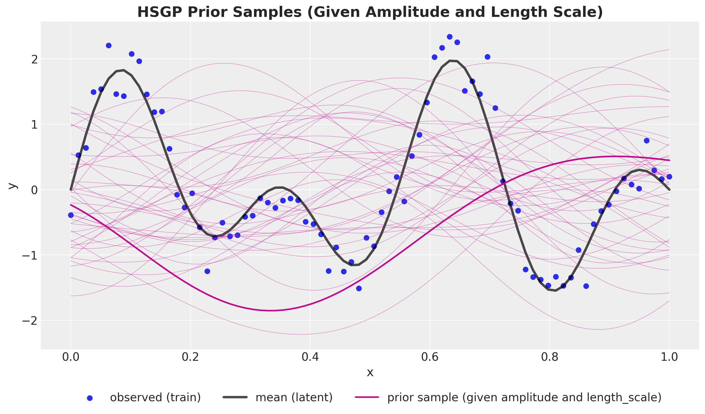
Prior Predictive
PyMC Implementation
HSGP Class
with pm.Model() as hsgp_pymc_model:
    x_data = pm.MutableData("x_data", value=x_train)
    y_data = pm.MutableData("y_data", y_train_obs)

    kernel_amplitude = pm.InverseGamma("kernel_amplitude", ...)
    kernel_length_scale = pm.InverseGamma("kernel_length_scale", ...)
    noise = pm.InverseGamma("noise", ...)

    mean = pm.gp.mean.Zero()
    cov = kernel_amplitude**2 * pm.gp.cov.ExpQuad(
        input_dim=1, ls=kernel_length_scale
    )
    gp = pm.gp.HSGP(m=[20], L=[1.3], mean_func=mean, cov_func=cov)
    f = gp.prior("f", X=x_data[:, None])

    pm.Normal("likelihood", mu=f, sigma=noise, observed=y_data)
Out-of-Sample Predictions
conditional method
with hsgp_pymc_model:
    x_star_data = pm.MutableData("x_star_data", x_test)
    f_star = gp.conditional("f_star", x_star_data[:, None])
    pm.set_data({"x_data": x_test, "y_data": np.ones_like(x_test)})
    hsgp_pymc_idata.extend(
        pm.sample_posterior_predictive(
            trace=hsgp_pymc_idata,
            var_names=["f_star", "likelihood"],
            random_seed=rng_subkey[1].item(),
        )
    )
HSGP Model - Posterior Predictive
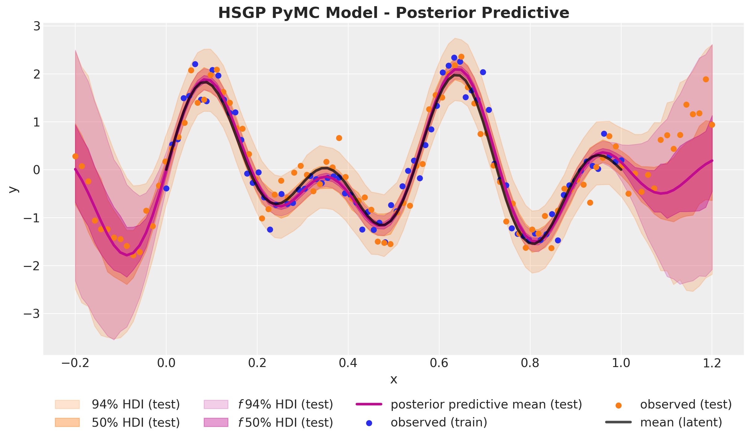
PyMC Implementation
HSGP.prior_linearized
with pm.Model() as hsgp_linearized_pymc_model:
    x_data = pm.MutableData("x_data", value=x_train)
    y_data = pm.MutableData("y_data", y_train_obs)

    kernel_amplitude = pm.InverseGamma("kernel_amplitude", ...)
    kernel_length_scale = pm.InverseGamma("kernel_length_scale", ...)
    noise = pm.InverseGamma("noise", ...)

    mean = pm.gp.mean.Zero()
    cov = kernel_amplitude**2 * pm.gp.cov.ExpQuad(input_dim=1, ls=kernel_length_scale)
    gp = pm.gp.HSGP(m=[20], L=[1.3], mean_func=mean, cov_func=cov)
    phi, sqrt_psd = gp.prior_linearized(Xs=x_data_centered[:, None])

    beta = pm.Normal("beta", mu=0, sigma=1, size=gp._m_star)
    f = pm.Deterministic("f", phi @ (beta * sqrt_psd))

    pm.Normal("likelihood", mu=f, sigma=noise, observed=y_data)
Out-of-Sample Predictions
pm.set_data method
Example: Birthdays Dataset
The Birthdays Dataset
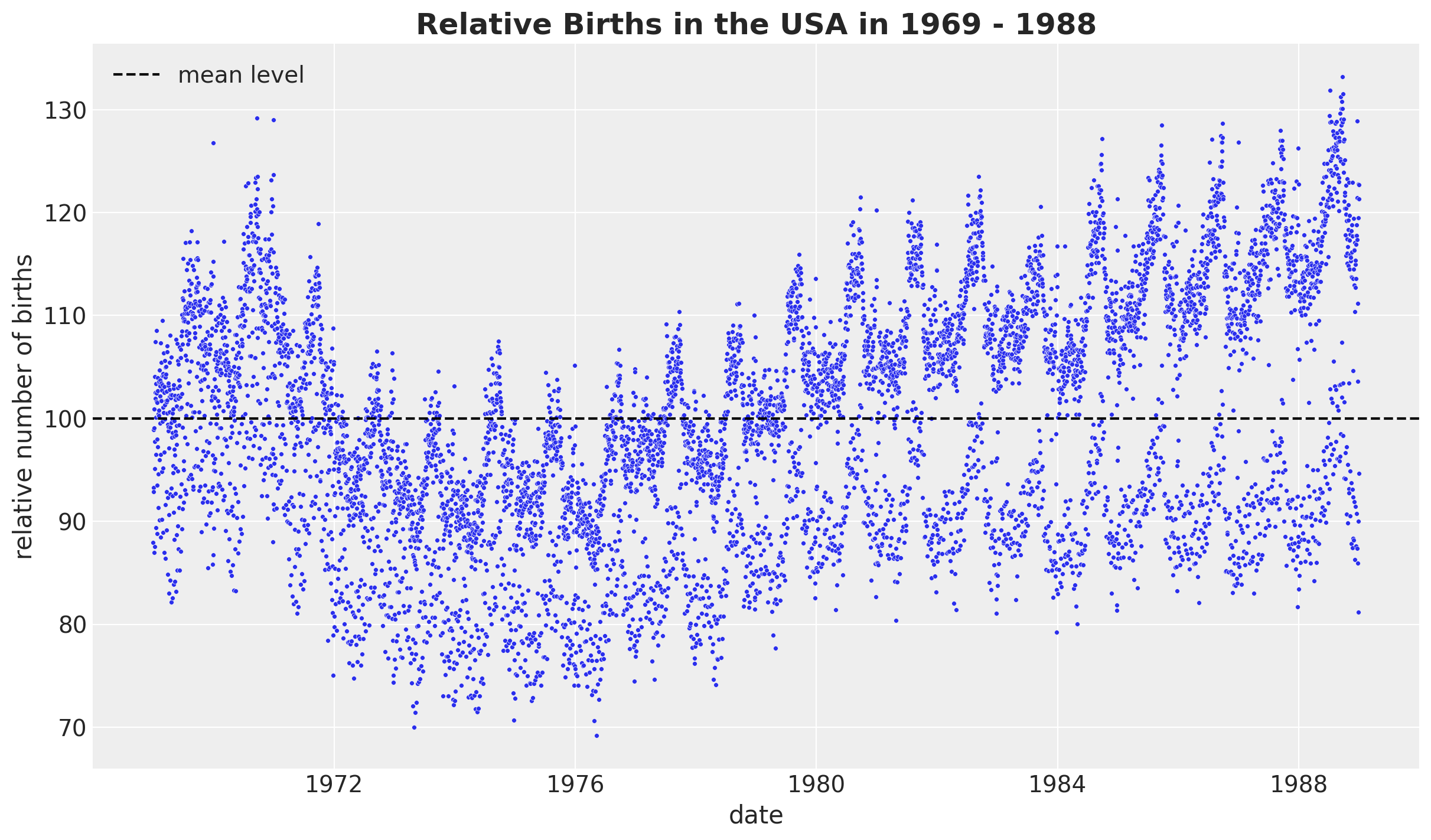
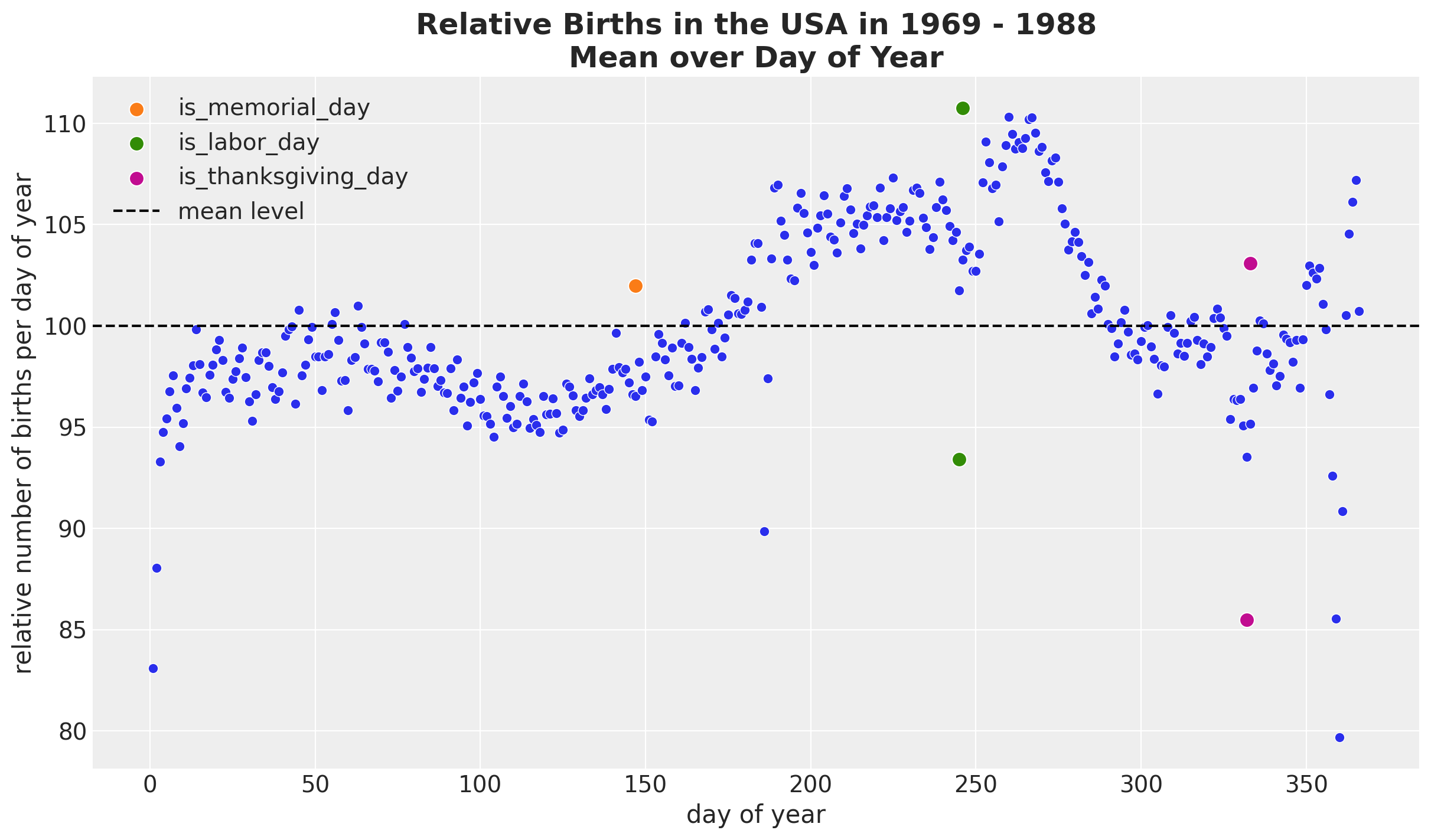
Seasonal Patterns - Day of Year
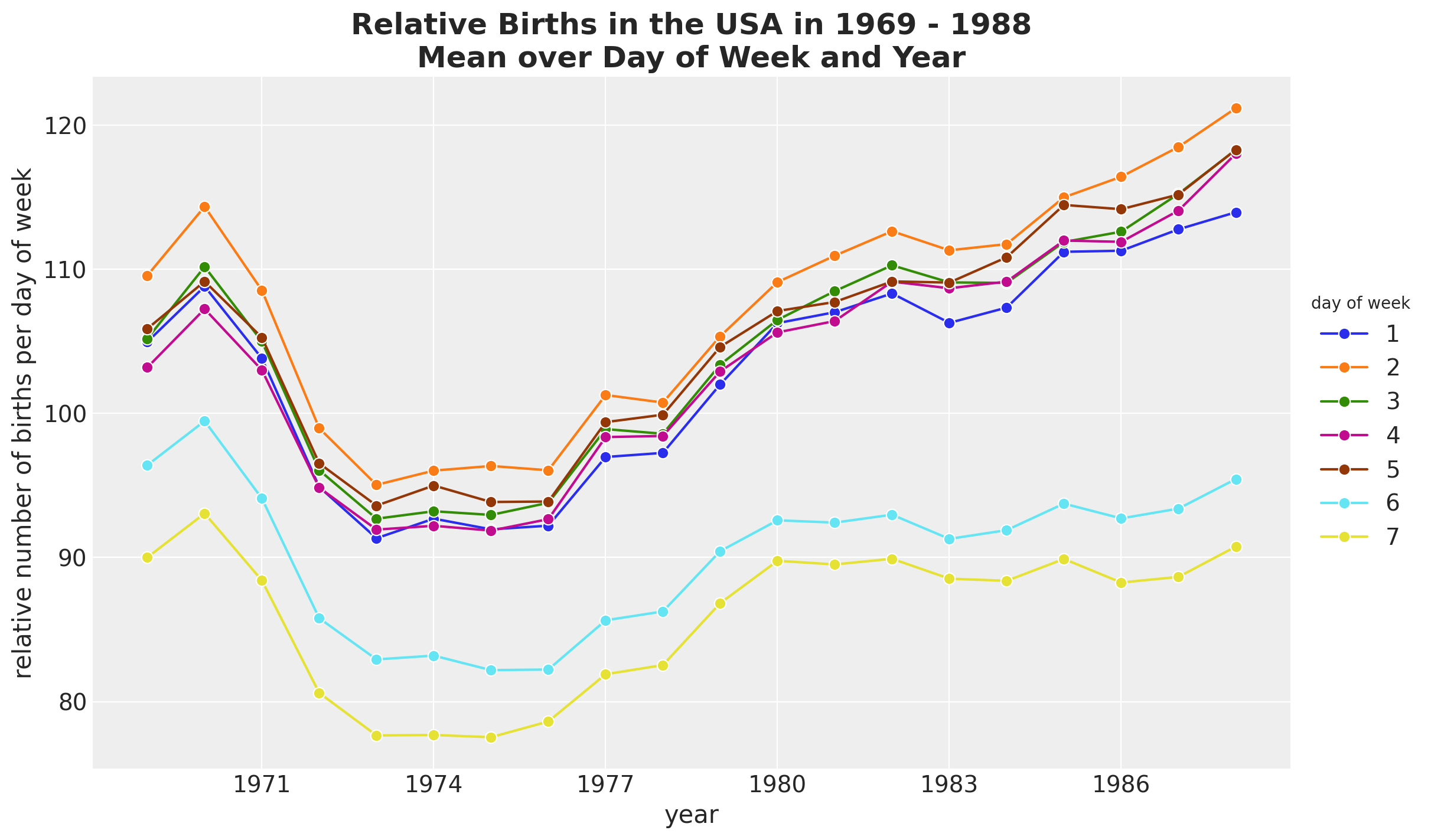
Seasonal Patterns - Day of Week
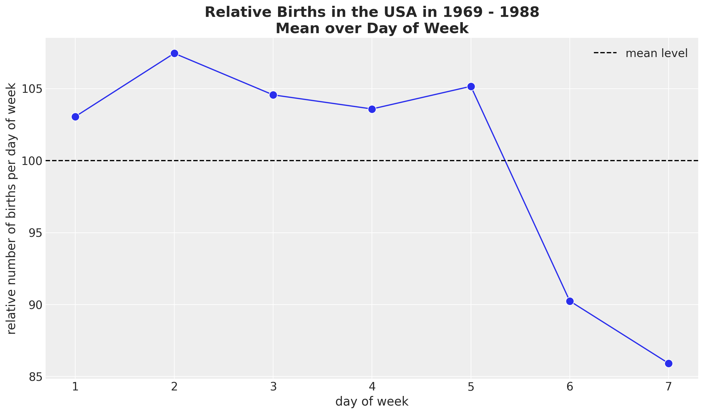
Seasonal Patterns - Day of Week
HSGP Model - Trend
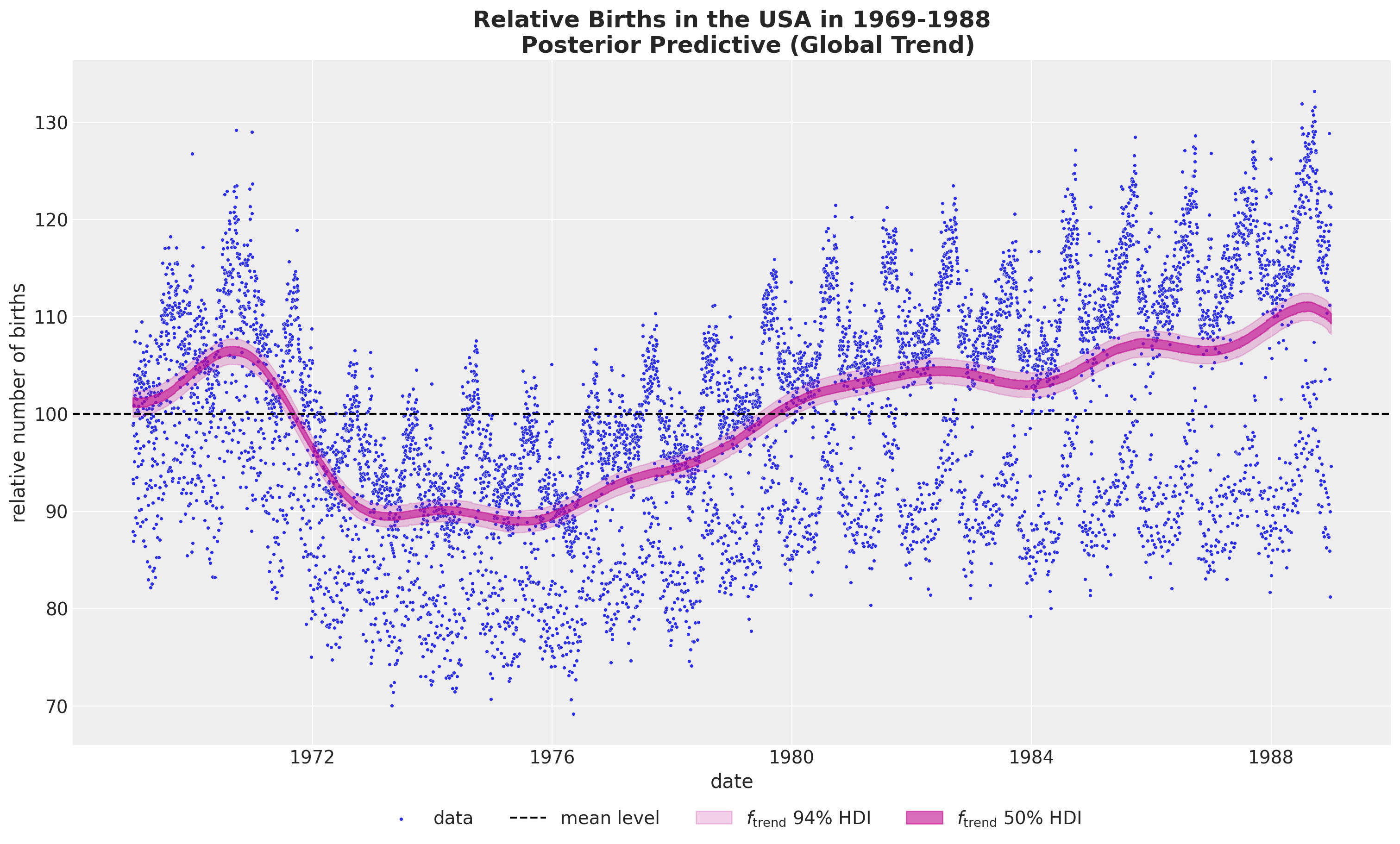
We use a Gaussian process with a squared exponential kernel.
HSGP Model - Yearly Seasonality
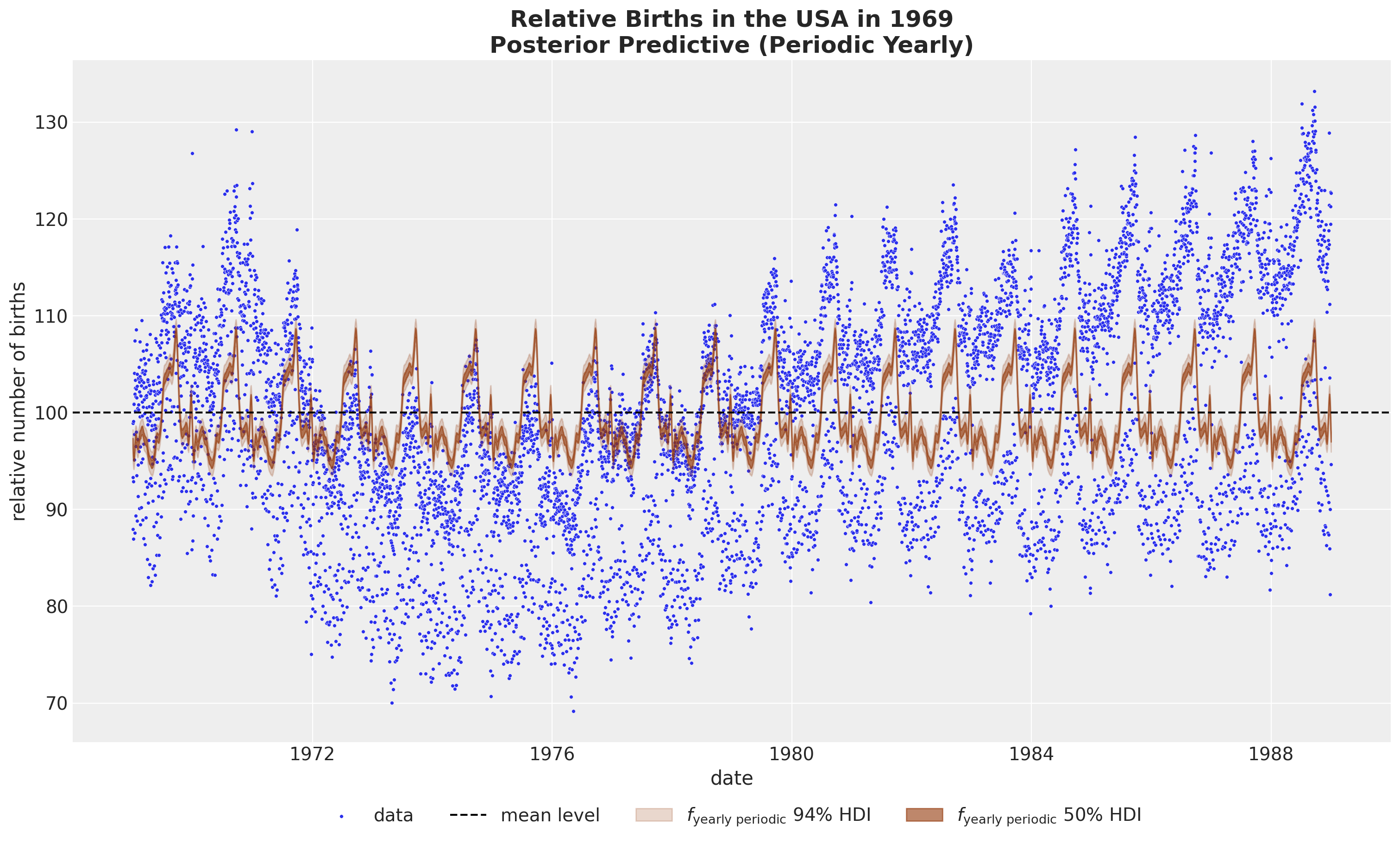
We use a Gaussian process with a periodic kernel*.
HSGP Model - Weekly Seasonality
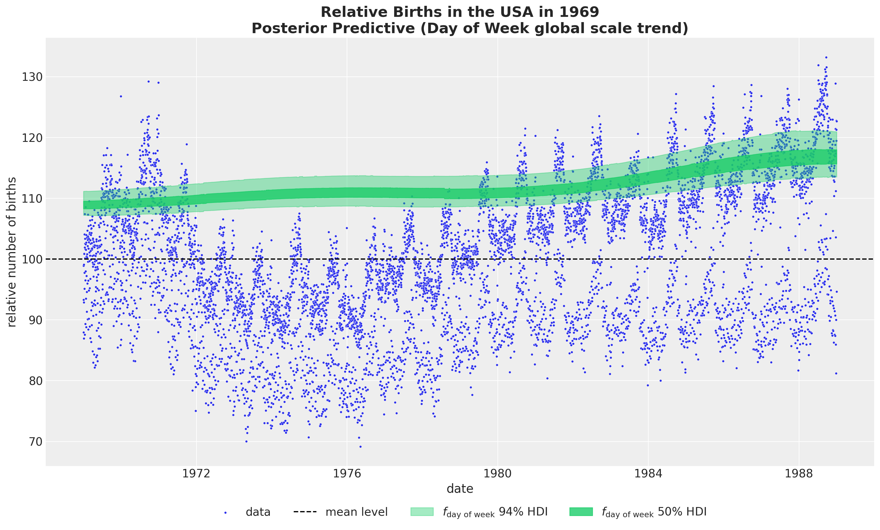
We use a ZeroSumNormal distribution to capture the relative difference across weekdays. We couple it with a multiplicative factor parametrized by a Gaussian process.
HSGP Model - Special Days
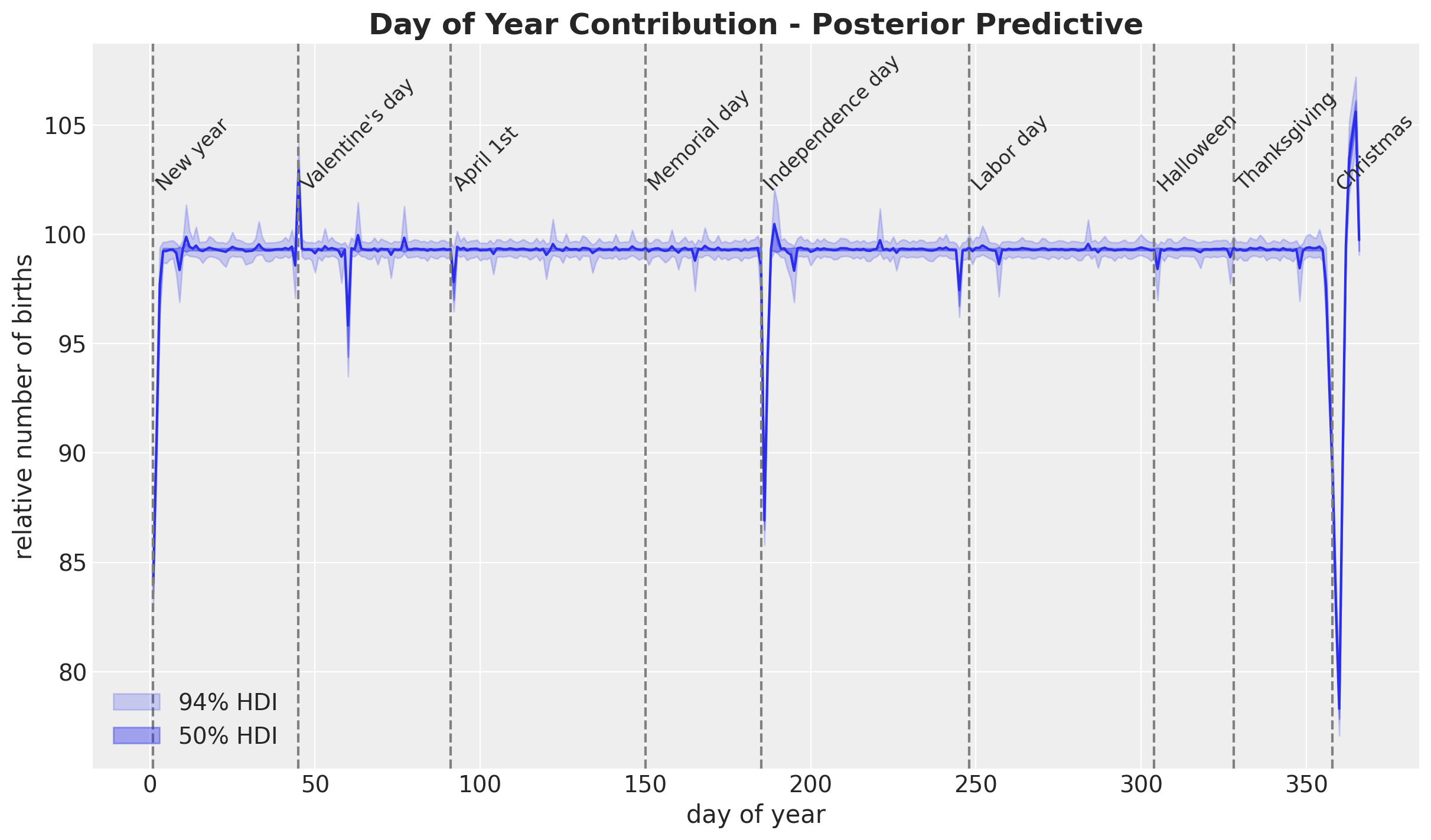
We use a StudentT distribution over the day_of_year2.
References
Gaussian Processes
- Gaussian Processes for Machine Learning, classic book on GPs.
- PyMC Examples: Mean and Covariance Functions
- Bayesian Regression as a Gaussian Process
- An Introduction to Gaussian Process Regression
- Robust Gaussian Process Modeling, very complete introduction to GPs.
- Dan Simpson’s Blog, many posts on GPs and prior selection.
HSGP Approximation
References
Birthdays Dataset
- Bayesian workflow book - Birthdays
- NumPyro Example: Hilbert space approximation for Gaussian processes
- Time Series Modeling with HSGP: Baby Births Example
Spectral Theory
Thank you!

