In this notebook, we extend the revenue-retention model introduced in the sequence of blog posts “Cohort Revenue & Retention Analysis: A Bayesian Approach” and “Cohort Revenue Retention Analysis with Flax and NumPyro” (plus the associated pre-print “Cohort Revenue & Retention Analysis: A Bayesian Approach”) to include analysis across different markets (or any type of grouping variable). The motivation for this extension is that in many real applications one is interested in understanding the revenue and retention patterns across different markets where typically we have different data sizes. Instead of modeling all separately, we take advantage of the hierarchical structure of the data to share information across markets. This will help have better forecasts for younger markets where limited data is available. We show through a simulation the power of this approach (and how relatively simple it is to implement once we have the basic model in place).
Prepare Notebook
from datetime import UTC, datetime
from itertools import pairwise

import arviz as az
import jax
import jax.numpy as jnp
import matplotlib.pyplot as plt
import matplotlib.ticker as mtick
import numpy as np
import numpyro
import numpyro.distributions as dist
import optax
import polars as pl
import seaborn as sns
from flax import nnx
from jax import random
from jaxtyping import Array, Float, Int
from numpyro.contrib.module import random_nnx_module
from numpyro.handlers import condition
from numpyro.infer import SVI, Trace_ELBO
from numpyro.infer.autoguide import AutoMultivariateNormal
from numpyro.infer.reparam import LocScaleReparam
from numpyro.infer.util import Predictive
from pydantic import BaseModel

# https://github.com/juanitorduz/website_projects/blob/master/Python/retention_data.py
from retention_data import CohortDataGenerator
from scipy.special import logit
from sklearn.compose import ColumnTransformer
from sklearn.pipeline import Pipeline
from sklearn.preprocessing import (
    LabelEncoder,
    OneHotEncoder,
    RobustScaler,
)

numpyro.set_host_device_count(n=4)

rng_key = random.PRNGKey(seed=42)

az.style.use("arviz-darkgrid")
plt.rcParams["figure.figsize"] = [12, 7]
plt.rcParams["figure.dpi"] = 100
plt.rcParams["figure.facecolor"] = "white"

%load_ext autoreload
%autoreload 2
%load_ext jaxtyping
%jaxtyping.typechecker beartype.beartype
%config InlineBackend.figure_format = "retina"
seed: int = sum(map(ord, "retention"))
rng: np.random.Generator = np.random.default_rng(seed=seed)Generate Data
We extend the data generating process from the previous post so that we can generate data for multiple markets. The code to generate data for one market is available in the retention_data.py file.
class Market(BaseModel):
    """Class to represent a market."""

    name: str
    start_date: datetime
    n_cohorts: int
    user_base: int = 10_000


class MarketDataGenerator:
    """Class to generate market data from the cohort data generator."""

    def __init__(self, markets: list[Market], rng: np.random.Generator) -> None:
        self.markets = markets
        self.rng = rng

    def run(self) -> pl.DataFrame:
        data_dfs: list[pl.DataFrame] = []

        for market in self.markets:
            cohort_generator = CohortDataGenerator(
                rng=self.rng, start_cohort=market.start_date, n_cohorts=market.n_cohorts
            )
            data_df = cohort_generator.run()

            # Add some features
            data_df = data_df.with_columns(
                (pl.col("n_active_users") / pl.col("n_users")).alias("retention"),
                pl.lit(market.name).alias("market"),
                (pl.col("cohort").dt.month()).alias("cohort_month"),
                (pl.col("period").dt.month()).alias("period_month"),
            )
            data_dfs.append(data_df)
        return pl.concat(data_dfs)


# Set up the markets.
markets: list[Market] = [
    Market(
        name="A",
        start_date=datetime(2020, 1, 1, tzinfo=UTC),
        n_cohorts=48,
        user_base=10_000,
    ),
    Market(
        name="B",
        start_date=datetime(2021, 2, 1, tzinfo=UTC),
        n_cohorts=35,
        user_base=12_000,
    ),
    Market(
        name="C",
        start_date=datetime(2022, 1, 1, tzinfo=UTC),
        n_cohorts=24,
        user_base=1_000,
    ),
    Market(
        name="D",
        start_date=datetime(2022, 7, 1, tzinfo=UTC),
        n_cohorts=18,
        user_base=500,
    ),
]

# Generate the data for each market.
n_markets = len(markets)
market_data_generator = MarketDataGenerator(markets=markets, rng=rng)
data_df = market_data_generator.run()

data_df.head()| cohort | n_users | period | age | cohort_age | retention_true_mu | retention_true | n_active_users | revenue | retention | market | cohort_month | period_month |
|---|---|---|---|---|---|---|---|---|---|---|---|---|
| 2020-01-01 | 150 | 2020-01-01 | 1430 | 0 | -1.807373 | 0.140956 | 150 | 14019.256906 | 1.0 | "A" | 1 | 1 |
| 2020-01-01 | 150 | 2020-02-01 | 1430 | 31 | -1.474736 | 0.186224 | 25 | 1886.501237 | 0.166667 | "A" | 1 | 2 |
| 2020-01-01 | 150 | 2020-03-01 | 1430 | 60 | -2.281286 | 0.092685 | 13 | 1098.136314 | 0.086667 | "A" | 1 | 3 |
| 2020-01-01 | 150 | 2020-04-01 | 1430 | 91 | -3.20661 | 0.038918 | 6 | 477.852458 | 0.04 | "A" | 1 | 4 |
| 2020-01-01 | 150 | 2020-05-01 | 1430 | 121 | -3.112983 | 0.042575 | 2 | 214.667937 | 0.013333 | "A" | 1 | 5 |
We verify that the data generation process is working as expected. For instance, we verify that the data has the same last period for each market.
assert (
    len(
        set(
            data_df.group_by("market")
            .agg(pl.col("period").max().alias("max_period"))["max_period"]
            .to_list()
        )
    )
    == 1
)
Remark [Outlier]: As we want to make sure that (1) the market \(A\) coincides with the data from the previous post and (2) the data generation process is reproducible and deterministic, we keep the same seed for the random number generator. In this case there are some outliers in the data for market \(B\), which we simply manually remove. The reason is that the cohort size is extremely small and in real applications we would probably remove it anyway (we could still keep it, but is just for illustration purposes).
# specific outlier condition
data_to_remove = pl.col("market").eq(pl.lit("B")) & pl.col("cohort").eq(
    pl.lit(datetime(2021, 2, 1, tzinfo=UTC))
)

data_df = data_df.filter(data_to_remove.not_())
Train-Test Split
Similar to the previous post, we split the data into a training and test set.
period_train_test_split = datetime(2022, 11, 1, tzinfo=UTC)

train_data_df = data_df.filter(pl.col("period") <= pl.lit(period_train_test_split))
test_data_df = data_df.filter(pl.col("period") > pl.lit(period_train_test_split))
test_data_df = test_data_df.filter(
    pl.col("cohort").is_in(train_data_df["cohort"].unique().to_list())
)
Data Visualization
Now we visualize the retention and revenue patterns for each market.
for market in markets:
    fig, ax = plt.subplots(figsize=(17, 9))

    (
        train_data_df.with_columns(
            pl.col("cohort").dt.strftime("%Y-%m").alias("cohort"),
            pl.col("period").dt.strftime("%Y-%m").alias("period"),
        )
        .filter(pl.col("cohort_age").ne(0) & pl.col("market").eq(market.name))
        .select(["cohort", "period", "retention"])
        .pivot(index="cohort", on="period", values="retention")
        .to_pandas()
        .set_index("cohort")
        .pipe(
            (sns.heatmap, "data"),
            cmap="viridis_r",
            linewidths=0.2,
            linecolor="black",
            annot=True,
            fmt="0.0%",
            cbar_kws={"format": mtick.FuncFormatter(func=lambda y, _: f"{y:0.0%}")},
            ax=ax,
        )
    )

    [tick.set_rotation(0) for tick in ax.get_yticklabels()]

    ax.set_title(f"Retention by Cohort and Period for Market {market.name}")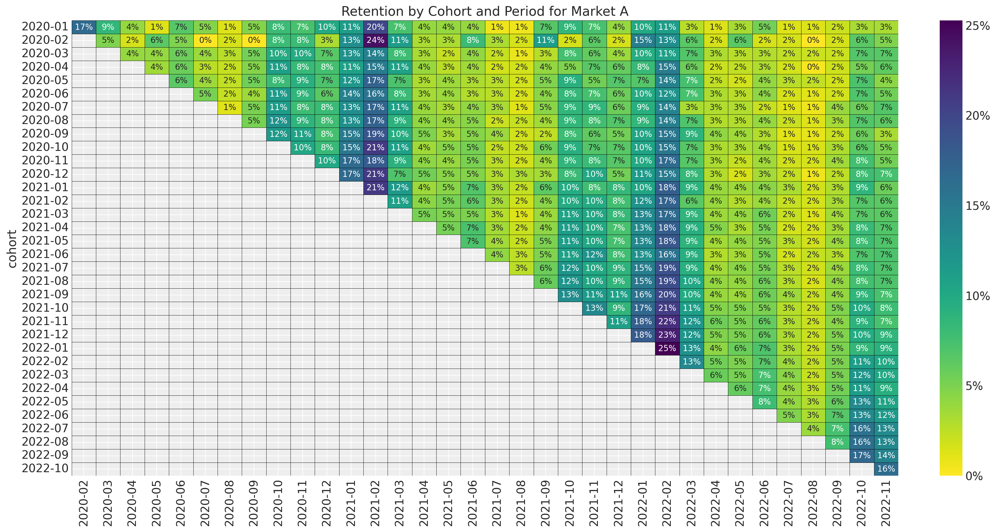
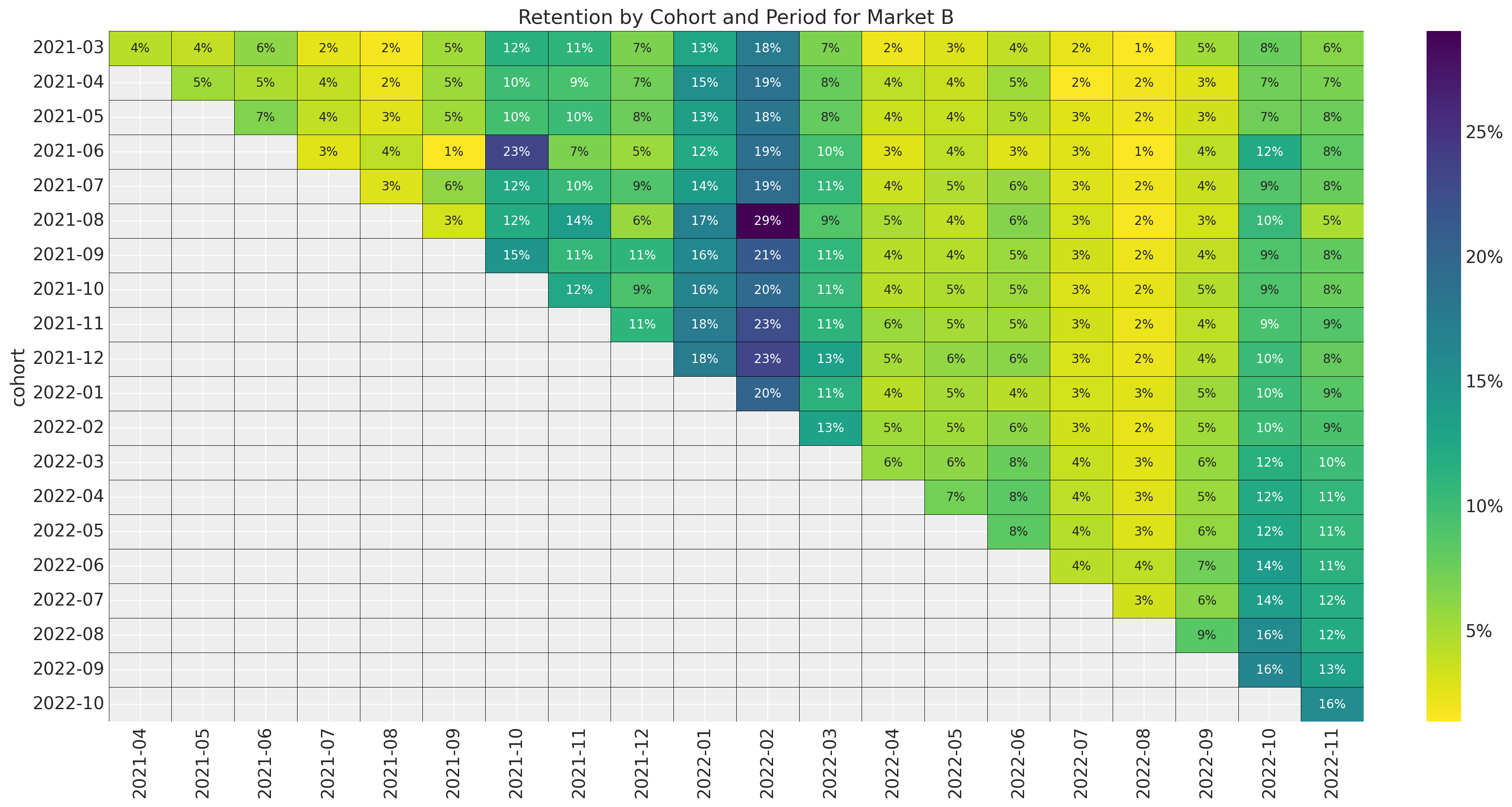
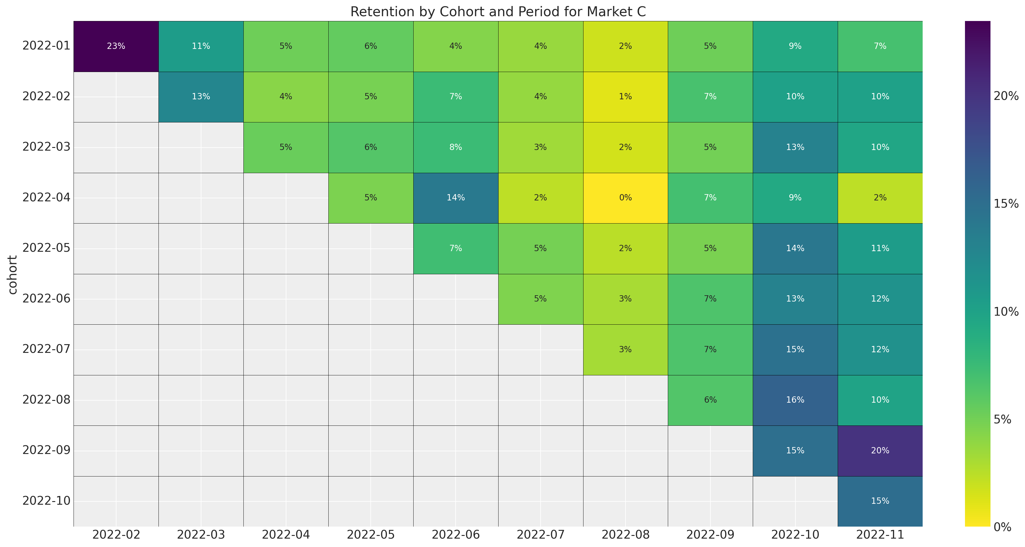
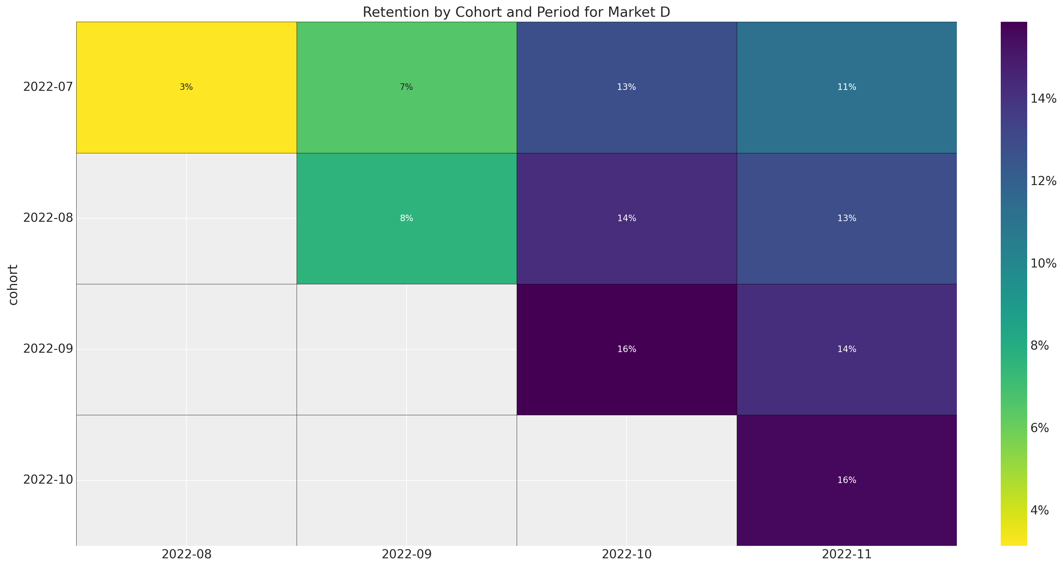
Here are some observations about the retention data:
- The data for market \(A\) is exactly the same as the data in the previous post.
- Note how market \(D\) has a much smaller number of cohorts than the other markets. It would be very hard to get any type of forecast for such a small cohort matrix by itself.
- All markets have strong seasonal patterns both in the cohort and period dimensions.
Now we look at the revenue data.
for market in markets:
    fig, ax = plt.subplots(figsize=(17, 9))

    (
        train_data_df.with_columns(
            pl.col("cohort").dt.strftime("%Y-%m").alias("cohort"),
            pl.col("period").dt.strftime("%Y-%m").alias("period"),
        )
        .filter(pl.col("cohort_age").ne(0) & pl.col("market").eq(market.name))
        .select(["cohort", "period", "revenue"])
        .pivot(index="cohort", on="period", values="revenue")
        .to_pandas()
        .set_index("cohort")
        .pipe(
            (sns.heatmap, "data"),
            cmap="viridis_r",
            linewidths=0.2,
            linecolor="black",
            cbar_kws={"format": mtick.FuncFormatter(func=lambda y, _: f"{y:0.0f}")},
            ax=ax,
        )
    )

    [tick.set_rotation(0) for tick in ax.get_yticklabels()]

    ax.set_title(f"Revenue by Cohort and Period for {market.name}")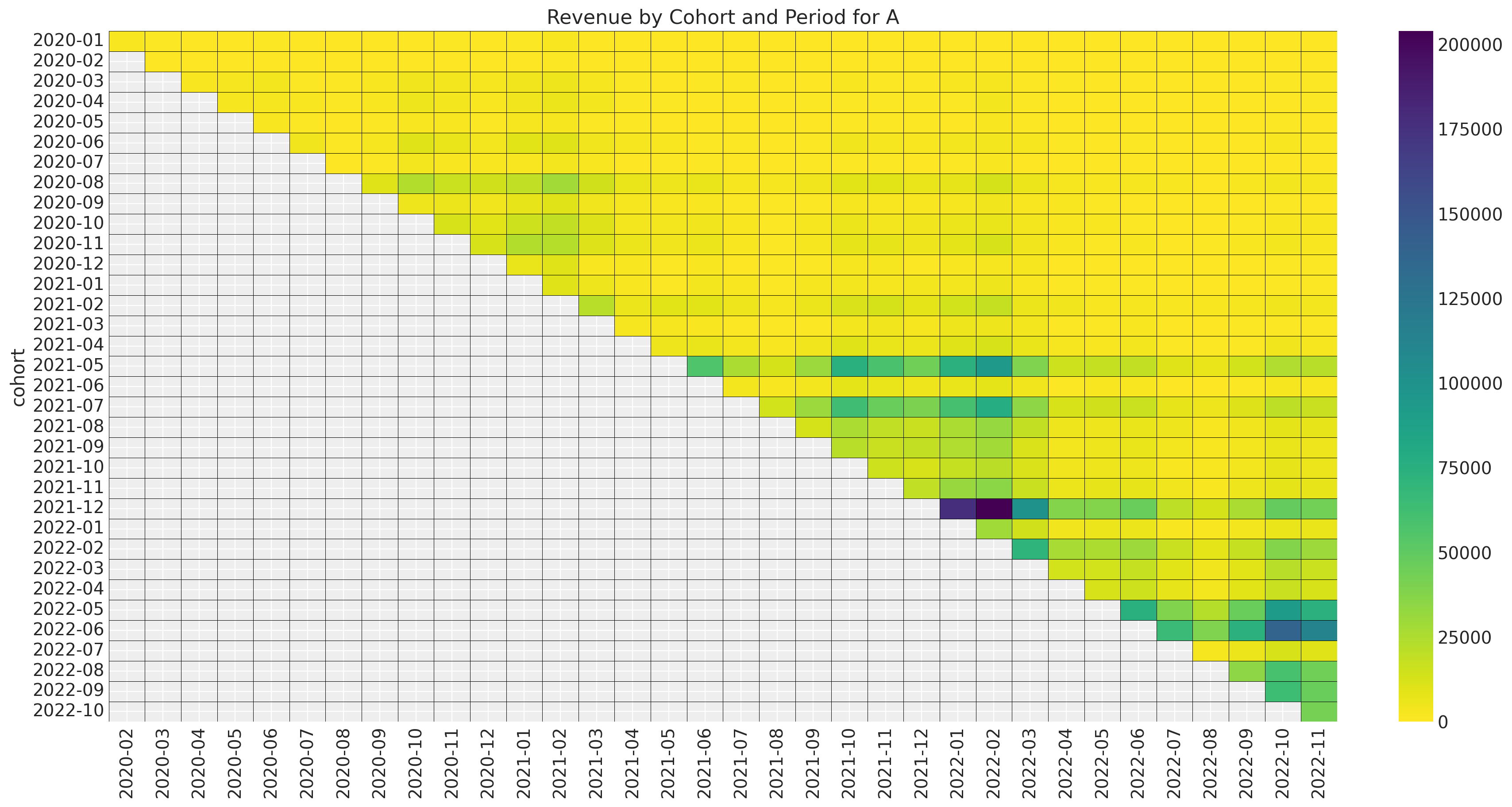
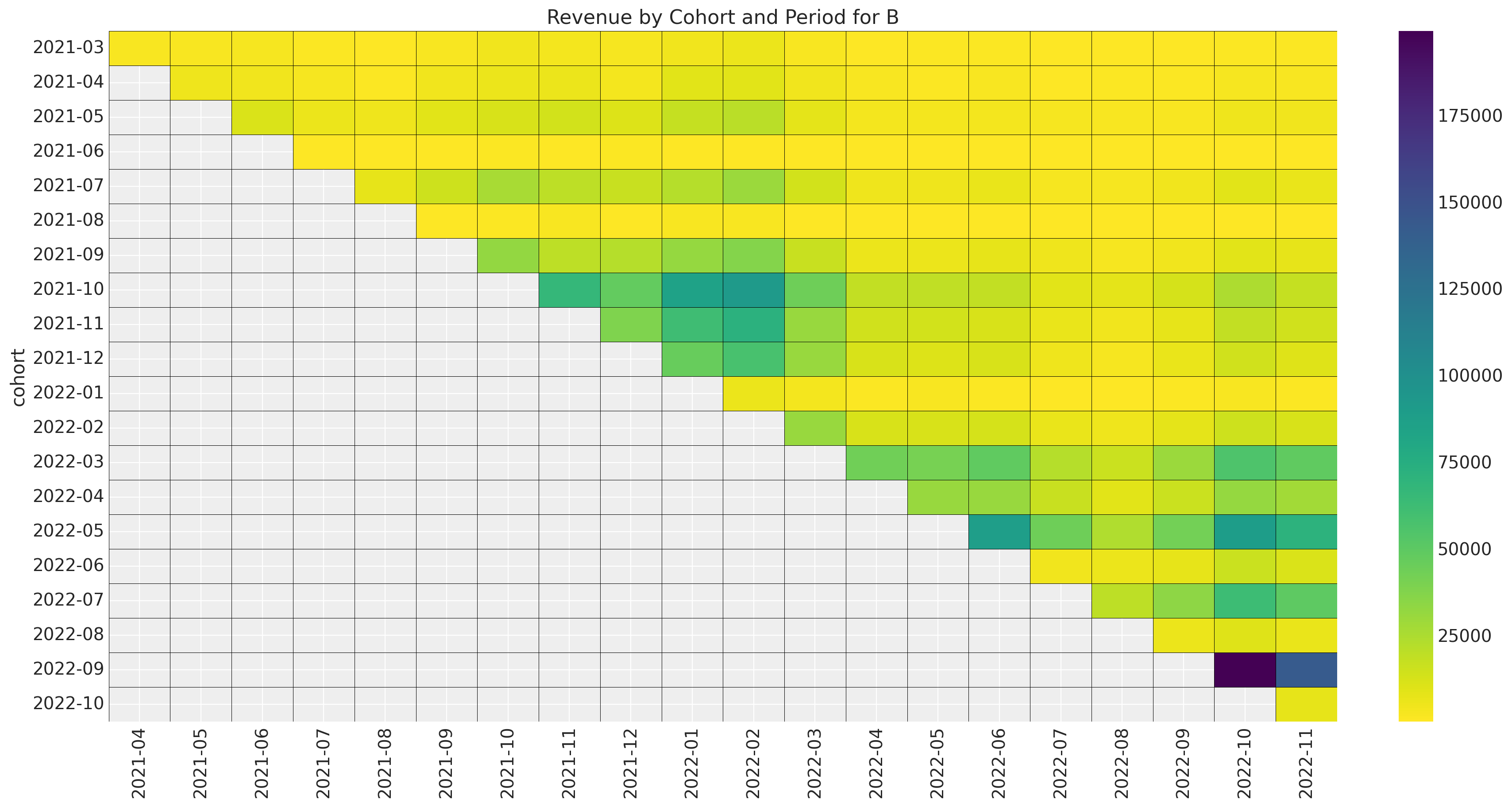
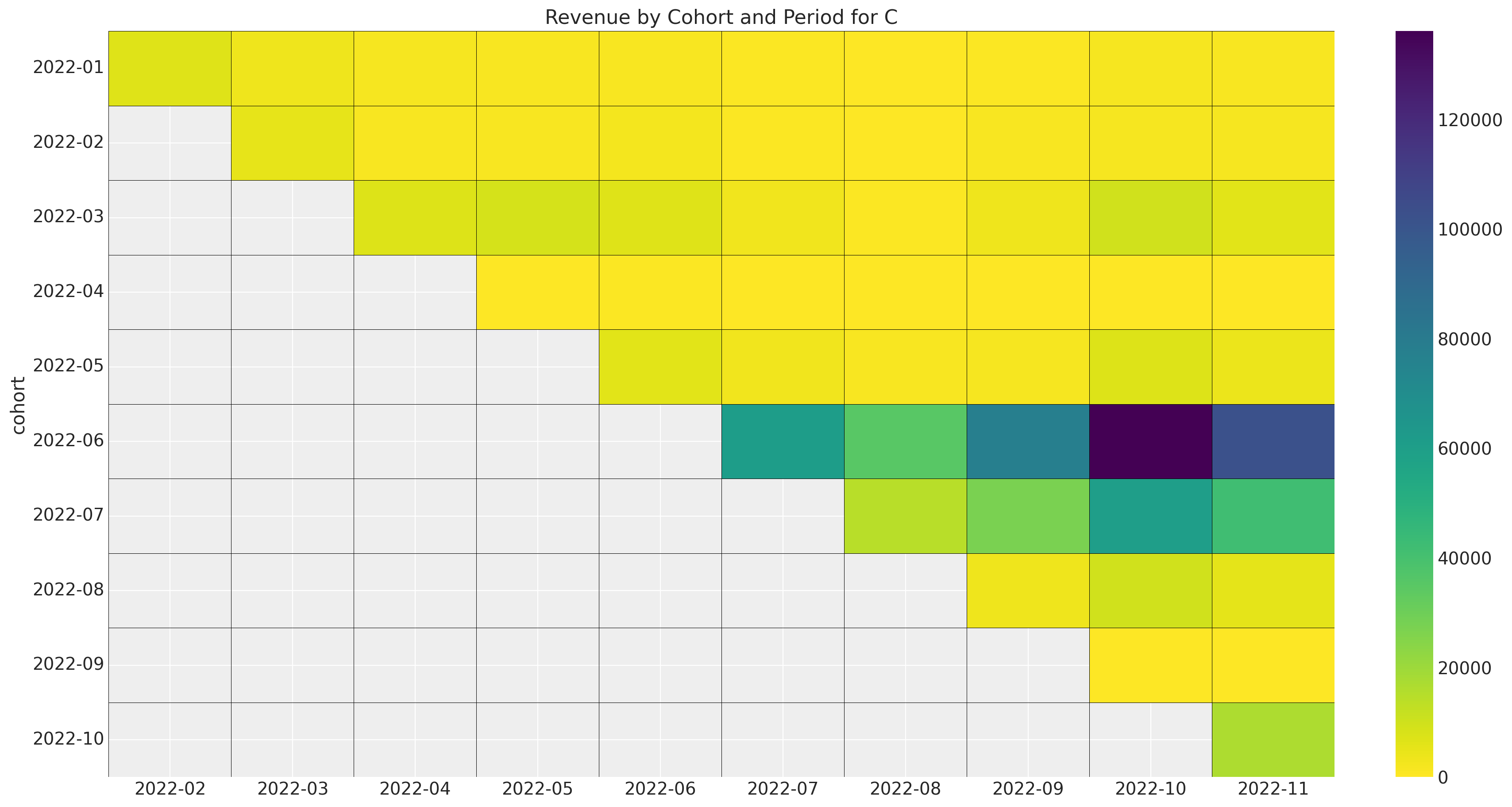
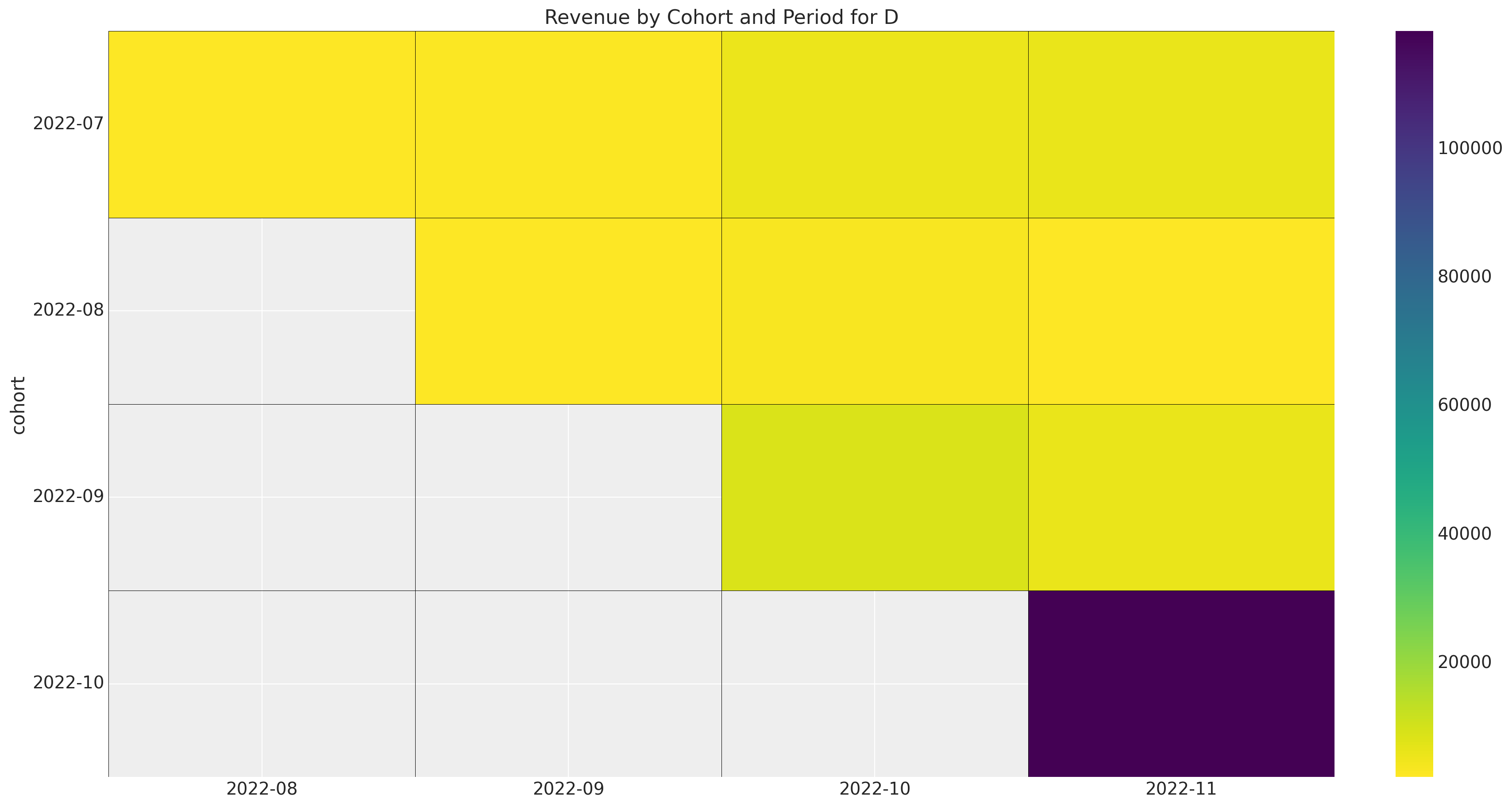
Overall, we see that the more recent cohorts account for a much larger fraction of the revenue than the older cohorts.
Data Pre-Processing
We continue with the data pre-processing step. All of the transformations are very standard: scaling for continuous variables, one-hot encoding for categorical variables, and label encoding for the cohort and period variables. For more details, see the previous post.
eps = np.finfo(float).eps

train_data_red_df = train_data_df.filter(pl.col("cohort_age").gt(pl.lit(0)))
train_obs_idx = jnp.array(range(train_data_red_df.shape[0]))
train_n_users = train_data_red_df["n_users"].to_jax()
train_n_active_users = train_data_red_df["n_active_users"].to_jax()
train_retention = train_data_red_df["retention"].to_jax()
train_retention_logit = logit(train_retention + eps)
train_revenue = train_data_red_df["revenue"].to_jax() + eps
train_revenue_per_user = train_revenue / (train_n_active_users + eps)

train_cohort = train_data_red_df["cohort"].to_numpy()
train_cohort_encoder = LabelEncoder()
train_cohort_idx = train_cohort_encoder.fit_transform(train_cohort).flatten()
train_period = train_data_red_df["period"].to_numpy()
train_period_encoder = LabelEncoder()
train_period_idx = train_period_encoder.fit_transform(train_period).flatten()
train_market = train_data_red_df["market"].to_numpy()
train_market_encoder = LabelEncoder()
train_market_idx = jnp.array(train_market_encoder.fit_transform(train_market).flatten())

features: list[str] = [
    "age",
    "cohort_age",
    "cohort_month",
    "period_month",
    "market",
]
x_train = train_data_red_df[features]

train_age = train_data_red_df["age"].to_jax()
train_age_scaler = RobustScaler()
train_age_scaled = jnp.array(
    train_age_scaler.fit_transform(np.array(train_age).reshape(-1, 1)).flatten()
)

train_cohort_age = train_data_red_df["cohort_age"].to_jax()
train_cohort_age_scaler = RobustScaler()
train_cohort_age_scaled = jnp.array(
    train_cohort_age_scaler.fit_transform(
        np.array(train_cohort_age).reshape(-1, 1)
    ).flatten()
)

numerical_features = ["age", "cohort_age", "cohort_month", "period_month"]
categorical_features = ["market"]

numerical_transformer = Pipeline(steps=[("scaler", RobustScaler())])
categorical_features_transformer = Pipeline(
    steps=[("onehot", OneHotEncoder(drop="first", sparse_output=False))]
)

preprocessor = ColumnTransformer(
    transformers=[
        ("num", numerical_transformer, numerical_features),
        ("cat", categorical_features_transformer, categorical_features),
    ]
).set_output(transform="polars")

preprocessor.fit(x_train)
x_train_preprocessed = preprocessor.transform(x_train)

x_train_preprocessed_array = x_train_preprocessed.to_jax()
Model Specification
We extend the model from the blog post “Cohort Revenue Retention Analysis with Flax and NumPyro”. Recall that the idea is to use a neural network to model the retention component and couple it with a linear model for the revenue component. There are many ways to encode the market feature (and this framework allows for many different ways to do so). Here we use the following encoding:
- In the retention component, we simply add the market as a feature.
- In the revenue component, where we use a linear model, we add a hierarchical structure on the regressors.
To make this model scalable to tens or hundreds of markets, we use stochastic variational inference (SVI) to fit the model. In the case of few markets, we can use MCMC to fit the model.
Let’s start by defining the retention neural network.
class RetentionMLP(nnx.Module):
    def __init__(
        self, din: int, dout: int, hidden_layers: list[int], *, rngs: nnx.Rngs
    ) -> None:
        self.layers = []
        layer_dims = [din, *hidden_layers, dout]
        for in_dim, out_dim in pairwise(layer_dims):
            self.layers.append(nnx.Linear(in_dim, out_dim, rngs=rngs))

    def __call__(self, x: Float[Array, "obs features"]) -> Float[Array, "obs 1"]:
        for layer in self.layers[:-1]:
            x = jax.nn.tanh(layer(x))
        return jax.nn.sigmoid(self.layers[-1](x))
We can initialize the NNX object.
rng_key, rng_subkey = random.split(rng_key)

retention_nnx_module = RetentionMLP(
    din=x_train_preprocessed_array.shape[1],
    dout=1,
    hidden_layers=[4, 2, 2, 1],
    rngs=nnx.Rngs(rng_subkey),
)
Now we are ready to specify the model in NumPyro.
def retention_component(x: Float[Array, "obs features"]) -> Float[Array, " obs"]:
    """Retention component of the model via a neural network."""

    retention_nn = random_nnx_module(
        "retention_nn",
        retention_nnx_module,
        prior=dist.SoftLaplace(loc=0, scale=1),
    )

    return numpyro.deterministic("retention", retention_nn(x).squeeze(-1))


def revenue_component(
    age: Float[Array, " obs"],
    cohort_age: Float[Array, " obs"],
    market_idx: Int[Array, " obs"],
) -> Float[Array, " obs"]:
    """Revenue component of the model via a hierarchical linear model."""
    n_markets: int = np.unique(market_idx).size

    # --- Priors ---

    ## --- Parameters ---
    market_intercept_loc = numpyro.sample(
        "market_intercept_loc", dist.Normal(loc=0, scale=1)
    )
    market_intercept_scale = numpyro.sample(
        "market_intercept_scale", dist.HalfNormal(scale=1)
    )

    market_b_age_loc = numpyro.sample("market_b_age_loc", dist.Normal(loc=0, scale=1))
    market_b_age_scale = numpyro.sample("market_b_age_scale", dist.HalfNormal(scale=1))

    market_b_cohort_age_loc = numpyro.sample(
        "market_b_cohort_age_loc", dist.Normal(loc=0, scale=1)
    )
    market_b_cohort_age_scale = numpyro.sample(
        "market_b_cohort_age_scale", dist.HalfNormal(scale=1)
    )

    market_b_interaction_loc = numpyro.sample(
        "market_b_interaction_loc", dist.Normal(loc=0, scale=1)
    )
    market_b_interaction_scale = numpyro.sample(
        "market_b_interaction_scale", dist.HalfNormal(scale=1)
    )

    ## --- Parametrization Factors ---
    market_intercept_centered = numpyro.sample(
        "market_intercept_centered", dist.Uniform(low=0, high=1)
    )
    market_b_age_centered = numpyro.sample(
        "market_b_age_centered", dist.Uniform(low=0, high=1)
    )
    market_b_cohort_age_centered = numpyro.sample(
        "market_b_cohort_age_centered", dist.Uniform(low=0, high=1)
    )
    market_b_interaction_centered = numpyro.sample(
        "market_b_interaction_centered", dist.Uniform(low=0, high=1)
    )

    with (
        numpyro.plate("markets", n_markets),
        numpyro.handlers.reparam(
            config={
                "market_intercept": LocScaleReparam(centered=market_intercept_centered),
            }
        ),
        numpyro.handlers.reparam(
            config={
                "market_b_age": LocScaleReparam(centered=market_b_age_centered),
            }
        ),
        numpyro.handlers.reparam(
            config={
                "market_b_cohort_age": LocScaleReparam(
                    centered=market_b_cohort_age_centered
                ),
            }
        ),
        numpyro.handlers.reparam(
            config={
                "market_b_interaction": LocScaleReparam(
                    centered=market_b_interaction_centered
                ),
            }
        ),
    ):
        market_intercept = numpyro.sample(
            "market_intercept",
            dist.Normal(loc=market_intercept_loc, scale=market_intercept_scale),
        )

        market_b_age = numpyro.sample(
            "market_b_age",
            dist.Normal(loc=market_b_age_loc, scale=market_b_age_scale),
        )

        market_b_cohort_age = numpyro.sample(
            "market_b_cohort_age",
            dist.Normal(loc=market_b_cohort_age_loc, scale=market_b_cohort_age_scale),
        )

        market_b_interaction = numpyro.sample(
            "market_b_interaction",
            dist.Normal(loc=market_b_interaction_loc, scale=market_b_interaction_scale),
        )

    ## --- Parametrization ---
    lam_raw = numpyro.deterministic(
        "lam_log",
        market_intercept[market_idx]
        + market_b_age[market_idx] * age
        + market_b_cohort_age[market_idx] * cohort_age
        + market_b_interaction[market_idx] * age * cohort_age,
    )

    return numpyro.deterministic("lam", jax.nn.softplus(lam_raw))


def model(
    x: Float[Array, "obs features"],
    age: Float[Array, " obs"],
    cohort_age: Float[Array, " obs"],
    n_users: Int[Array, " obs"],
    market_idx: Int[Array, " obs"],
) -> None:
    """Hierarchical revenue-retention model."""

    n_obs: int = x.shape[0]

    retention = retention_component(x=x)
    lam = revenue_component(age=age, cohort_age=cohort_age, market_idx=market_idx)

    with numpyro.plate("data", n_obs):
        n_active_users = numpyro.sample(
            "n_active_users",
            dist.Binomial(total_count=n_users, probs=retention),
        )

        numpyro.deterministic("retention_estimated", n_active_users / n_users)

        numpyro.sample(
            "revenue",
            dist.Gamma(concentration=n_active_users + eps, rate=lam),
        )
Note that the hierarchical extension is relatively straightforward. One has to be careful with the dimensions (as always). Let’s now visualize the model structure:
numpyro.render_model(
    model=model,
    model_kwargs={
        "x": x_train_preprocessed_array,
        "age": train_age_scaled,
        "cohort_age": train_cohort_age_scaled,
        "n_users": train_n_users,
        "market_idx": train_market_idx,
    },
    render_distributions=True,
    render_params=True,
)
We proceed to condition the model on the data.
conditioned_model = condition(
    model,
    {"n_active_users": train_n_active_users, "revenue": train_revenue},
)
Stochastic Variational Inference
Having defined the model, we now fit it using SVI. We use some custom optimizers to speed up the inference (see optax documentation for more details).
# See https://optax.readthedocs.io/en/latest/getting_started.html#custom-optimizers
scheduler = optax.linear_onecycle_schedule(
    transition_steps=50_000,
    peak_value=0.01,
    pct_start=0.01,
    pct_final=0.75,
    div_factor=2,
    final_div_factor=3,
)

optimizer = optax.chain(
    optax.clip_by_global_norm(1.0),
    optax.scale_by_adam(),
    optax.scale_by_schedule(scheduler),
    optax.scale(-1.0),
)

guide = AutoMultivariateNormal(model=conditioned_model)

svi = SVI(conditioned_model, guide, optimizer, loss=Trace_ELBO())
n_samples = 50_000
rng_key, rng_subkey = random.split(key=rng_key)
svi_result = svi.run(
    rng_subkey,
    n_samples,
    x=x_train_preprocessed_array,
    age=train_age_scaled,
    cohort_age=train_cohort_age_scaled,
    n_users=train_n_users,
    market_idx=train_market_idx,
)

fig, ax = plt.subplots(figsize=(9, 6))
ax.plot(svi_result.losses)
ax.set(yscale="log")
ax.set_title("ELBO Loss", fontsize=18, fontweight="bold");
100%|██████████| 50000/50000 [00:11<00:00, 4420.64it/s, init loss: 9282986.0000, avg. loss [47501-50000]: 9852.0283] 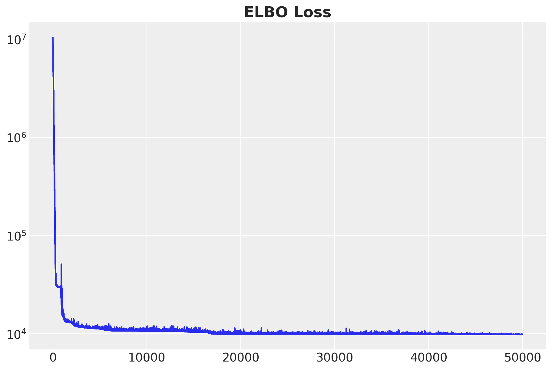
Overall, the ELBO curve looks good. We continue to sample from the posterior distribution.
params = svi_result.params

posterior_predictive = Predictive(
    model=model,
    guide=guide,
    params=params,
    num_samples=4 * 2_000,
    return_sites=[
        "retention",
        "n_active_users",
        "revenue",
        "retention_estimated",
    ],
)
rng_key, rng_subkey = random.split(key=rng_key)
posterior_predictive_samples = posterior_predictive(
    rng_subkey,
    x_train_preprocessed_array,
    train_age_scaled,
    train_cohort_age_scaled,
    train_n_users,
    train_market_idx,
)
We store the samples in an az.InferenceData object.
idata = az.from_dict(
    posterior_predictive={
        k: np.expand_dims(a=np.asarray(v), axis=0)
        for k, v in posterior_predictive_samples.items()
    },
    coords={"obs_idx": train_obs_idx},
    dims={
        "retention": ["obs_idx"],
        "n_active_users": ["obs_idx"],
        "revenue": ["obs_idx"],
        "retention_estimated": ["obs_idx"],
    },
)
In-Sample Predictions
Now that we have fit the model, we can make in-sample predictions and compare them to the true values. Let’s start by plotting the posterior predictive distribution (and mean) of the retention.
fig, ax = plt.subplots(figsize=(9, 7))
sns.scatterplot(
    x=train_retention,
    y=idata["posterior_predictive"]["retention"].mean(dim=["chain", "draw"]),
    color="C0",
    label="Mean Predicted Retention",
    ax=ax,
)
az.plot_hdi(
    x=train_retention,
    y=idata["posterior_predictive"]["retention_estimated"],
    hdi_prob=0.94,
    color="C0",
    fill_kwargs={"alpha": 0.2, "label": "$94\\%$ HDI"},
    ax=ax,
)
az.plot_hdi(
    x=train_retention,
    y=idata["posterior_predictive"]["retention_estimated"],
    hdi_prob=0.5,
    color="C0",
    fill_kwargs={"alpha": 0.4, "label": "$50\\%$ HDI"},
    ax=ax,
)
sns.rugplot(x=train_retention, color="C0", ax=ax)
ax.axline((0, 0), slope=1, color="black", linestyle="--", label="diagonal")
ax.legend(loc="upper left")
ax.set(xlabel="True Retention", ylabel="Predicted Retention")
ax.set_title(
    label="True vs Predicted Retention (Train)", fontsize=18, fontweight="bold"
);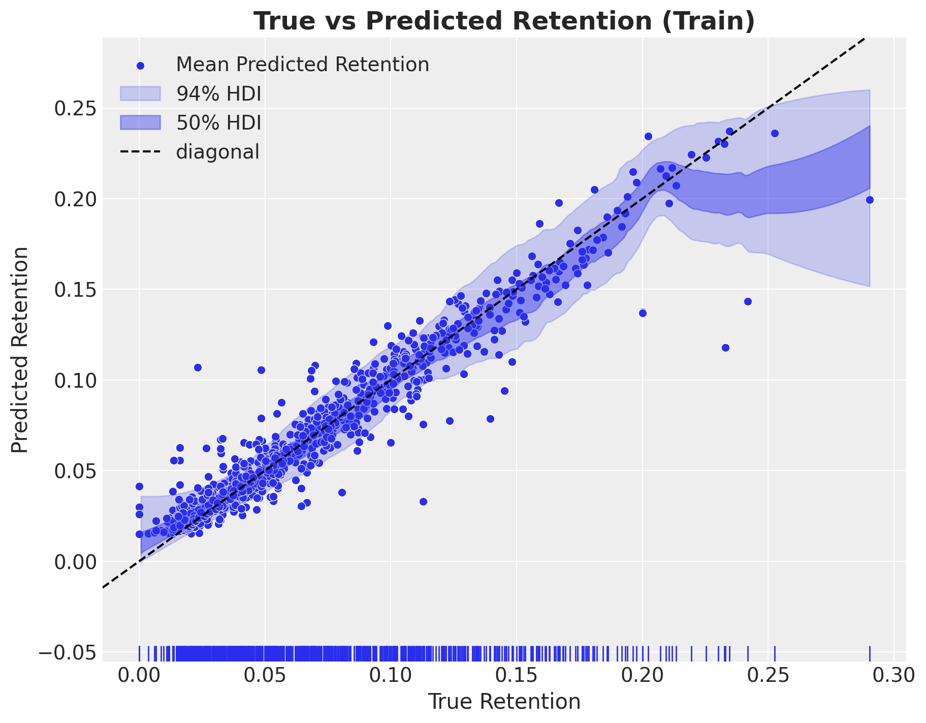
The model does a good job for the vast majority of the data. There are a few data points on which the model underpredicts the retention.
Next, we look into the analoge of the in-sample predictions for the revenue.
fig, ax = plt.subplots(figsize=(9, 7))
sns.scatterplot(
    x=train_revenue,
    y=idata["posterior_predictive"]["revenue"].mean(dim=["chain", "draw"]),
    color="C0",
    label="Mean Predicted Revenue",
    ax=ax,
)
az.plot_hdi(
    x=train_revenue,
    y=idata["posterior_predictive"]["revenue"],
    hdi_prob=0.94,
    color="C0",
    fill_kwargs={"alpha": 0.2, "label": "$94\\%$ HDI"},
    ax=ax,
)
az.plot_hdi(
    x=train_revenue,
    y=idata["posterior_predictive"]["revenue"],
    hdi_prob=0.5,
    color="C0",
    fill_kwargs={"alpha": 0.4, "label": "$50\\%$ HDI"},
    ax=ax,
)
sns.rugplot(x=train_revenue, color="C0", ax=ax)
ax.axline((0, 0), slope=1, color="black", linestyle="--", label="diagonal")
ax.legend(loc="upper left")
ax.set(xlabel="True Revenue", ylabel="Predicted Revenue")
ax.set_title(label="True vs Predicted Revenue (Train)", fontsize=18, fontweight="bold");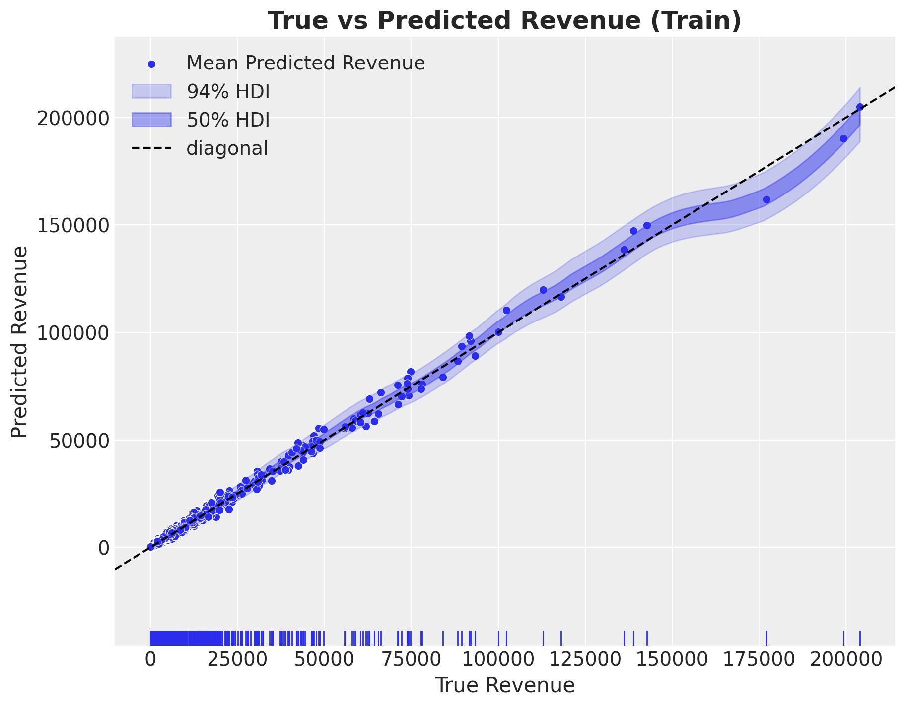
The revenue component has a very good in sample fit.
Retention
We now deep-dive into the retention component of the model. We look at specific cohorts to see how well the model is able to capture the variation in the retention patterns. For this, we define some helper functions to plot the retention patterns (similar to the ones we used in the previous posts).
train_retention_estimated_hdi = az.hdi(
    ary=idata["posterior_predictive"], hdi_prob=0.94
)["retention_estimated"]


def plot_train_retention_hdi_cohort(
    market: str, cohort: datetime, ax: plt.Axes
) -> plt.Axes:
    cohort_index = train_cohort_encoder.transform([cohort.replace(tzinfo=None)])[0]
    market_index = train_market_encoder.transform([market])[0]

    mask = (train_cohort_idx == cohort_index) & (
        np.array(train_market_idx) == market_index
    )

    ax.fill_between(
        x=train_period[train_period_idx[mask]],
        y1=train_retention_estimated_hdi[mask, :][:, 0],
        y2=train_retention_estimated_hdi[mask, :][:, 1],
        alpha=0.2,
        color="C2",
        label="94% HDI",
    )
    sns.lineplot(
        x=train_period[train_period_idx[mask]],
        y=idata["posterior_predictive"]["retention"].mean(dim=["chain", "draw"])[mask],
        marker="o",
        color="C2",
        label="predicted",
        ax=ax,
    )

    sns.lineplot(
        x=train_period[train_period_idx[mask]],
        y=train_retention[mask],
        color="C0",
        marker="o",
        label="observed",
        ax=ax,
    )
    cohort_name = train_cohort_encoder.classes_[cohort_index]
    ax.legend(loc="upper left")
    ax.set(title=f"Cohort {cohort_name}")
    return ax
We now plot the in-sample estimated retentions for some selected cohorts and for all the markets.
cohorts_to_plot = [
    datetime(2020, 1, 1, tzinfo=UTC),
    datetime(2020, 2, 1, tzinfo=UTC),
    datetime(2020, 6, 1, tzinfo=UTC),
    datetime(2020, 11, 1, tzinfo=UTC),
    datetime(2021, 4, 1, tzinfo=UTC),
    datetime(2021, 9, 1, tzinfo=UTC),
    datetime(2022, 2, 1, tzinfo=UTC),
    datetime(2022, 7, 1, tzinfo=UTC),
    datetime(2022, 8, 1, tzinfo=UTC),
    datetime(2022, 9, 1, tzinfo=UTC),
]

fig, axes = plt.subplots(
    nrows=np.ceil(len(cohorts_to_plot) / 2).astype(int),
    ncols=2,
    figsize=(17, 11),
    sharex=True,
    sharey=True,
    layout="constrained",
)

for cohort, ax in zip(cohorts_to_plot, axes.flatten(), strict=True):
    plot_train_retention_hdi_cohort(market="A", cohort=cohort, ax=ax)
    ax.legend(loc="upper left")

fig.suptitle("In-Sample Retention - Market A", y=1.03, fontsize=20, fontweight="bold")
fig.autofmt_xdate()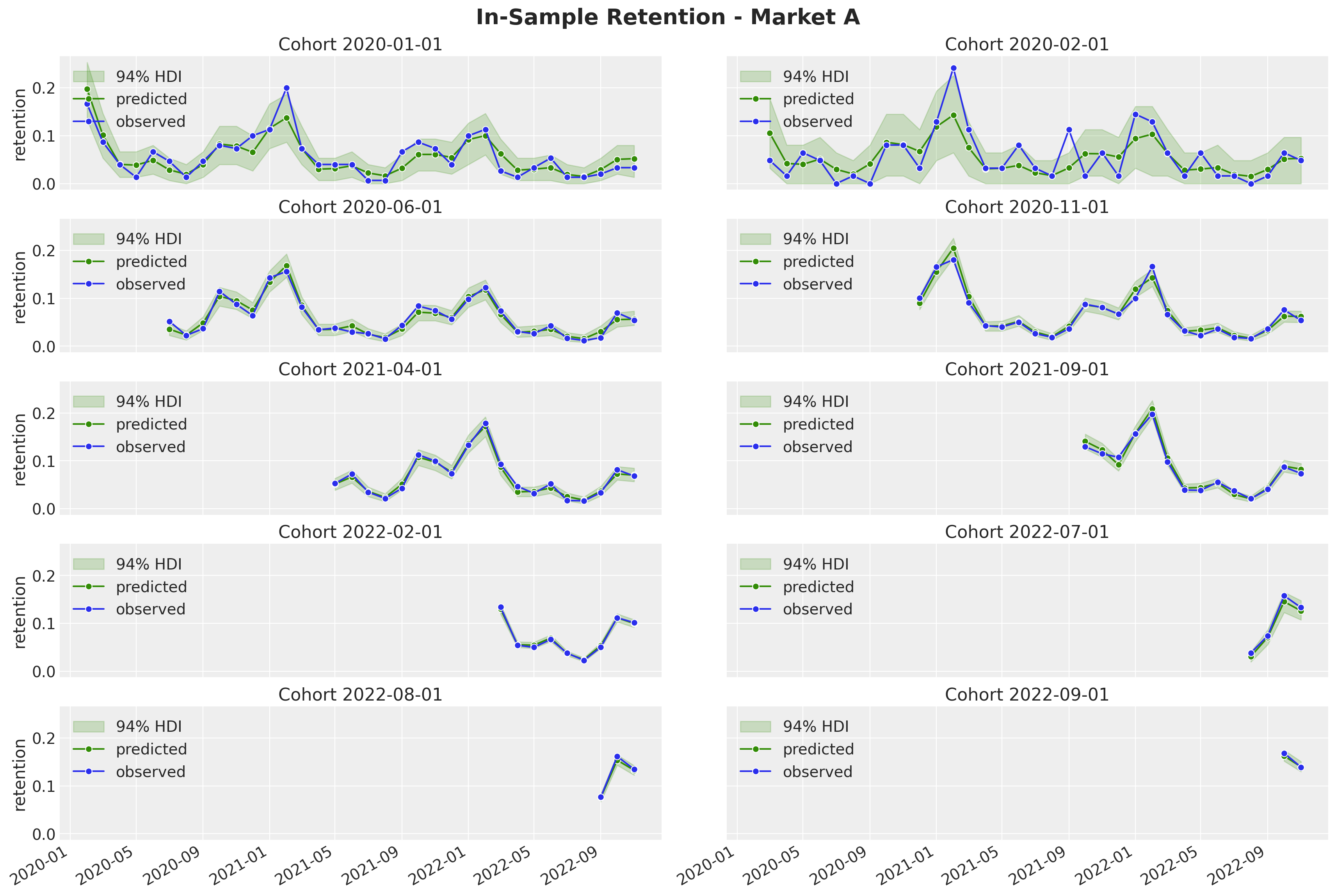
cohorts_to_plot = [
    datetime(2022, 3, 1, tzinfo=UTC),
    datetime(2022, 4, 1, tzinfo=UTC),
    datetime(2022, 5, 1, tzinfo=UTC),
    datetime(2022, 6, 1, tzinfo=UTC),
    datetime(2022, 7, 1, tzinfo=UTC),
    datetime(2022, 8, 1, tzinfo=UTC),
    datetime(2022, 9, 1, tzinfo=UTC),
    datetime(2022, 10, 1, tzinfo=UTC),
]

fig, axes = plt.subplots(
    nrows=np.ceil(len(cohorts_to_plot) / 2).astype(int),
    ncols=2,
    figsize=(17, 11),
    sharex=True,
    sharey=True,
    layout="constrained",
)

for cohort, ax in zip(cohorts_to_plot, axes.flatten(), strict=True):
    plot_train_retention_hdi_cohort(market="B", cohort=cohort, ax=ax)
    ax.legend(loc="upper left")

fig.suptitle("In-Sample Retention - Market B", y=1.03, fontsize=20, fontweight="bold")
fig.autofmt_xdate()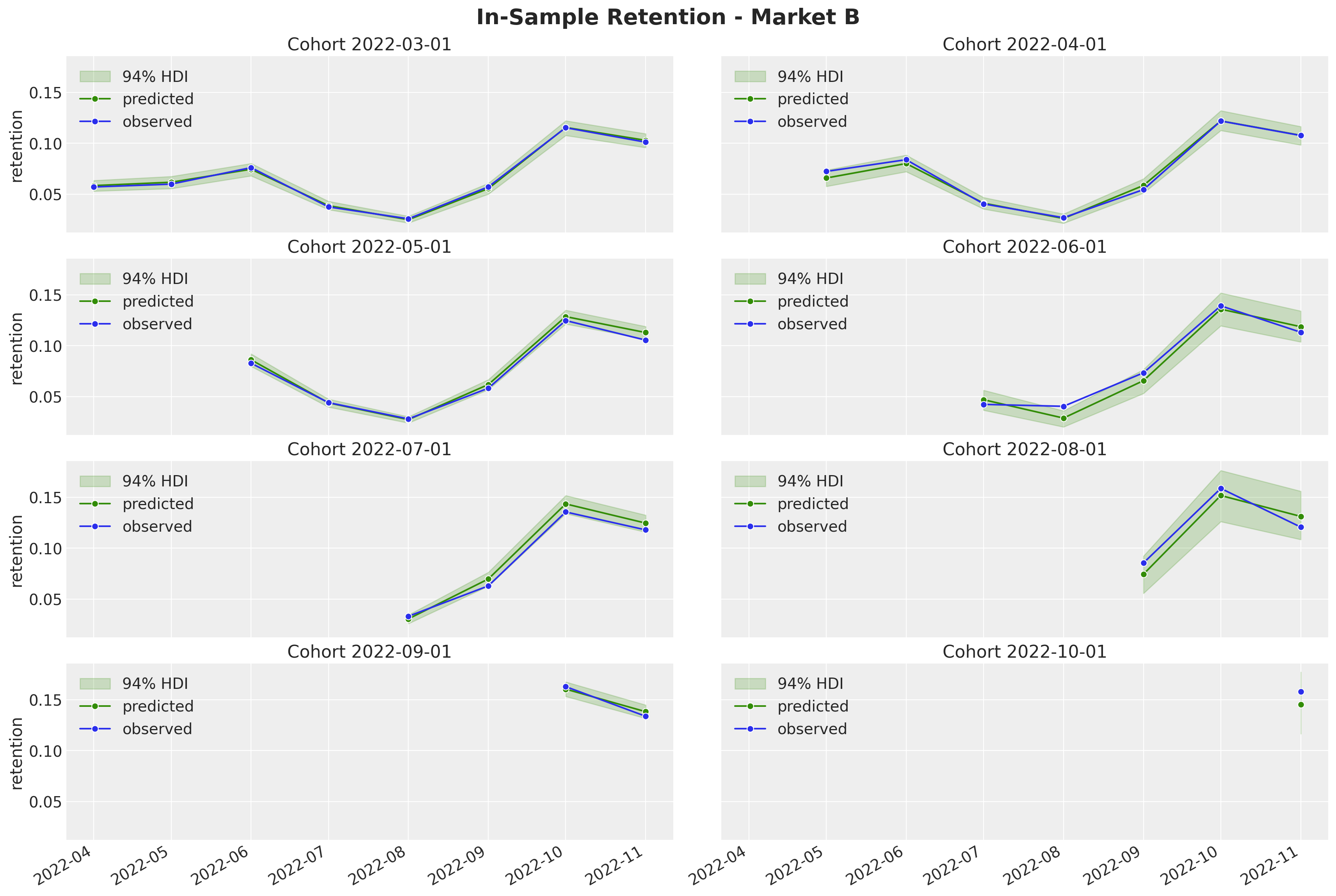
cohorts_to_plot = [
    datetime(2022, 3, 1, tzinfo=UTC),
    datetime(2022, 4, 1, tzinfo=UTC),
    datetime(2022, 5, 1, tzinfo=UTC),
    datetime(2022, 6, 1, tzinfo=UTC),
    datetime(2022, 7, 1, tzinfo=UTC),
    datetime(2022, 8, 1, tzinfo=UTC),
    datetime(2022, 9, 1, tzinfo=UTC),
    datetime(2022, 10, 1, tzinfo=UTC),
]

fig, axes = plt.subplots(
    nrows=np.ceil(len(cohorts_to_plot) / 2).astype(int),
    ncols=2,
    figsize=(17, 11),
    sharex=True,
    sharey=True,
    layout="constrained",
)

for cohort, ax in zip(cohorts_to_plot, axes.flatten(), strict=True):
    plot_train_retention_hdi_cohort(market="C", cohort=cohort, ax=ax)
    ax.legend(loc="upper left")

fig.suptitle("In-Sample Retention - Market C", y=1.03, fontsize=20, fontweight="bold")
fig.autofmt_xdate()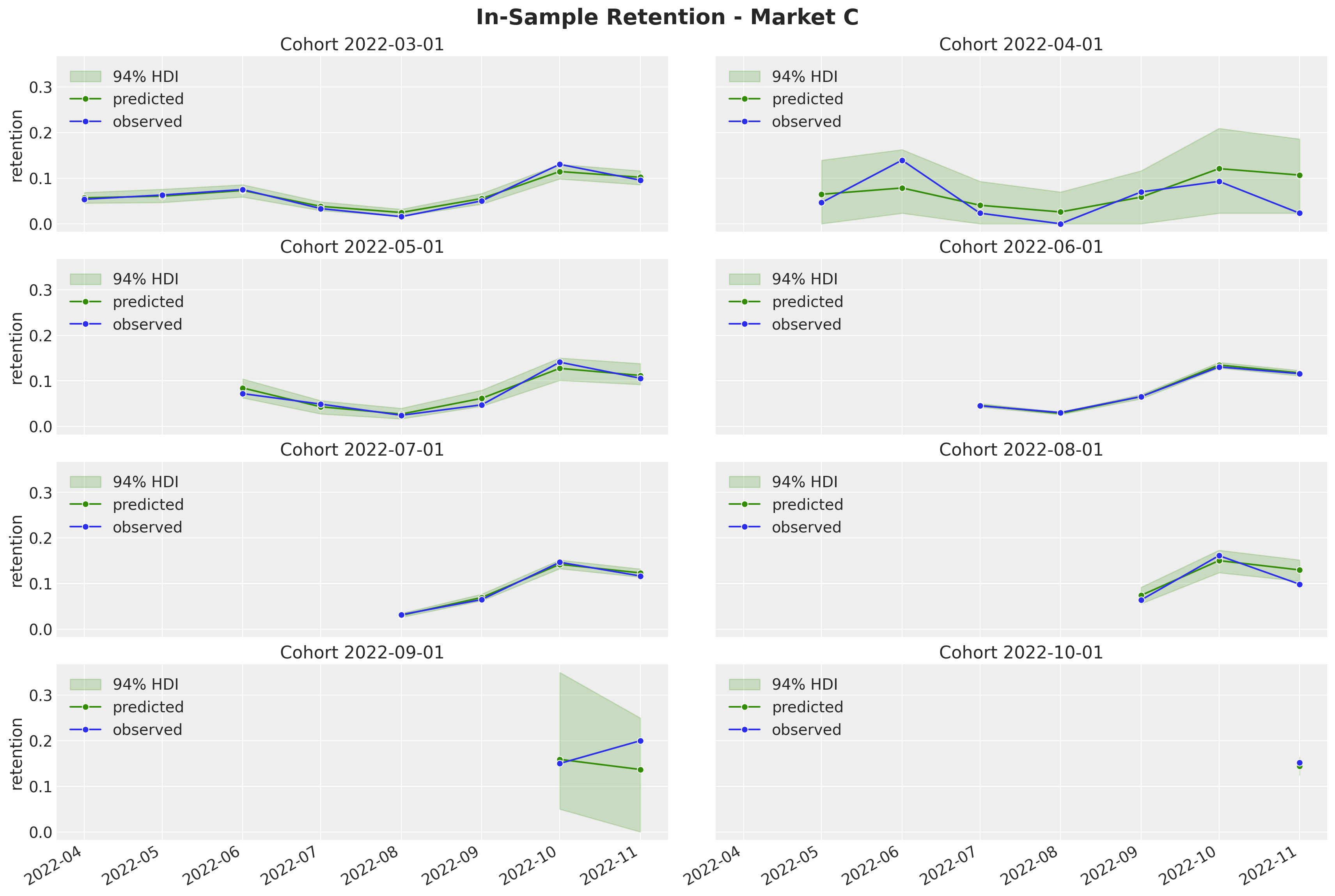
cohorts_to_plot = [
    datetime(2022, 7, 1, tzinfo=UTC),
    datetime(2022, 8, 1, tzinfo=UTC),
    datetime(2022, 9, 1, tzinfo=UTC),
    datetime(2022, 10, 1, tzinfo=UTC),
]

fig, axes = plt.subplots(
    nrows=np.ceil(len(cohorts_to_plot) / 2).astype(int),
    ncols=2,
    figsize=(17, 9),
    sharex=True,
    sharey=True,
    layout="constrained",
)

for cohort, ax in zip(cohorts_to_plot, axes.flatten(), strict=True):
    plot_train_retention_hdi_cohort(market="D", cohort=cohort, ax=ax)
    ax.legend(loc="upper left")

fig.suptitle("In-Sample Retention - Market D", y=1.03, fontsize=20, fontweight="bold")
fig.autofmt_xdate()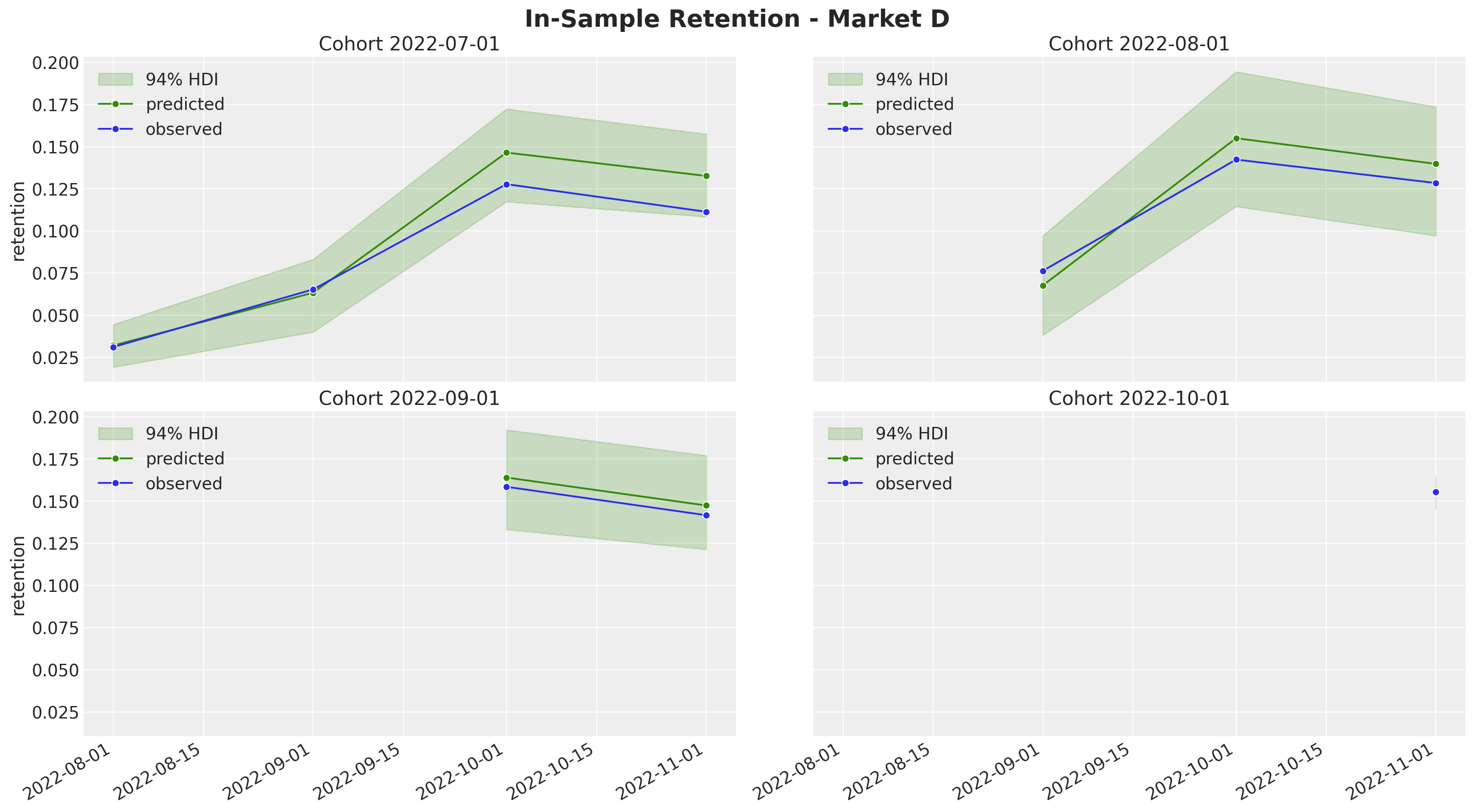
Overall, the model is able to capture the variation and trends of the retention component. Note, as expected, that the highest-density-intervals (HDI) for the smaller cohorts are wider than for the larger cohorts. This is by design, as we are modeling this retention component as a latent variable instead of modeling the quotients directly.
Revenue
We do the same for the revenue component.
train_revenue_hdi = az.hdi(ary=idata["posterior_predictive"], hdi_prob=0.94)["revenue"]


def plot_train_revenue_hdi_cohort(
    market: str, cohort: datetime, ax: plt.Axes
) -> plt.Axes:
    cohort_index = train_cohort_encoder.transform([cohort.replace(tzinfo=None)])[0]
    market_index = train_market_encoder.transform([market])[0]

    mask = (train_cohort_idx == cohort_index) & (
        np.array(train_market_idx) == market_index
    )

    ax.fill_between(
        x=train_period[train_period_idx[mask]],
        y1=train_revenue_hdi[mask, :][:, 0],
        y2=train_revenue_hdi[mask, :][:, 1],
        alpha=0.2,
        color="C3",
        label="94% HDI",
    )
    sns.lineplot(
        x=train_period[train_period_idx[mask]],
        y=idata["posterior_predictive"]["revenue"].mean(dim=["chain", "draw"])[mask],
        marker="o",
        color="C3",
        label="predicted",
        ax=ax,
    )

    sns.lineplot(
        x=train_period[train_period_idx[mask]],
        y=train_revenue[mask],
        color="C0",
        marker="o",
        label="observed",
        ax=ax,
    )
    cohort_name = train_cohort_encoder.classes_[cohort_index]
    ax.legend(loc="upper left")
    ax.set(title=f"Cohort {cohort_name}")
    return ax
cohorts_to_plot = [
datetime(2020, 1, 1, tzinfo=UTC),
datetime(2020, 2, 1, tzinfo=UTC),
datetime(2020, 6, 1, tzinfo=UTC),
datetime(2020, 11, 1, tzinfo=UTC),
datetime(2021, 4, 1, tzinfo=UTC),
datetime(2021, 9, 1, tzinfo=UTC),
datetime(2022, 2, 1, tzinfo=UTC),
datetime(2022, 7, 1, tzinfo=UTC),
datetime(2022, 8, 1, tzinfo=UTC),
datetime(2022, 9, 1, tzinfo=UTC),
]
fig, axes = plt.subplots(
nrows=np.ceil(len(cohorts_to_plot) / 2).astype(int),
ncols=2,
figsize=(17, 11),
sharex=True,
sharey=False,
layout="constrained",
)
for cohort, ax in zip(cohorts_to_plot, axes.flatten(), strict=True):
plot_train_revenue_hdi_cohort(market="A", cohort=cohort, ax=ax)
fig.suptitle("In-Sample Revenue - Market A", y=1.03, fontsize=20, fontweight="bold")
fig.autofmt_xdate()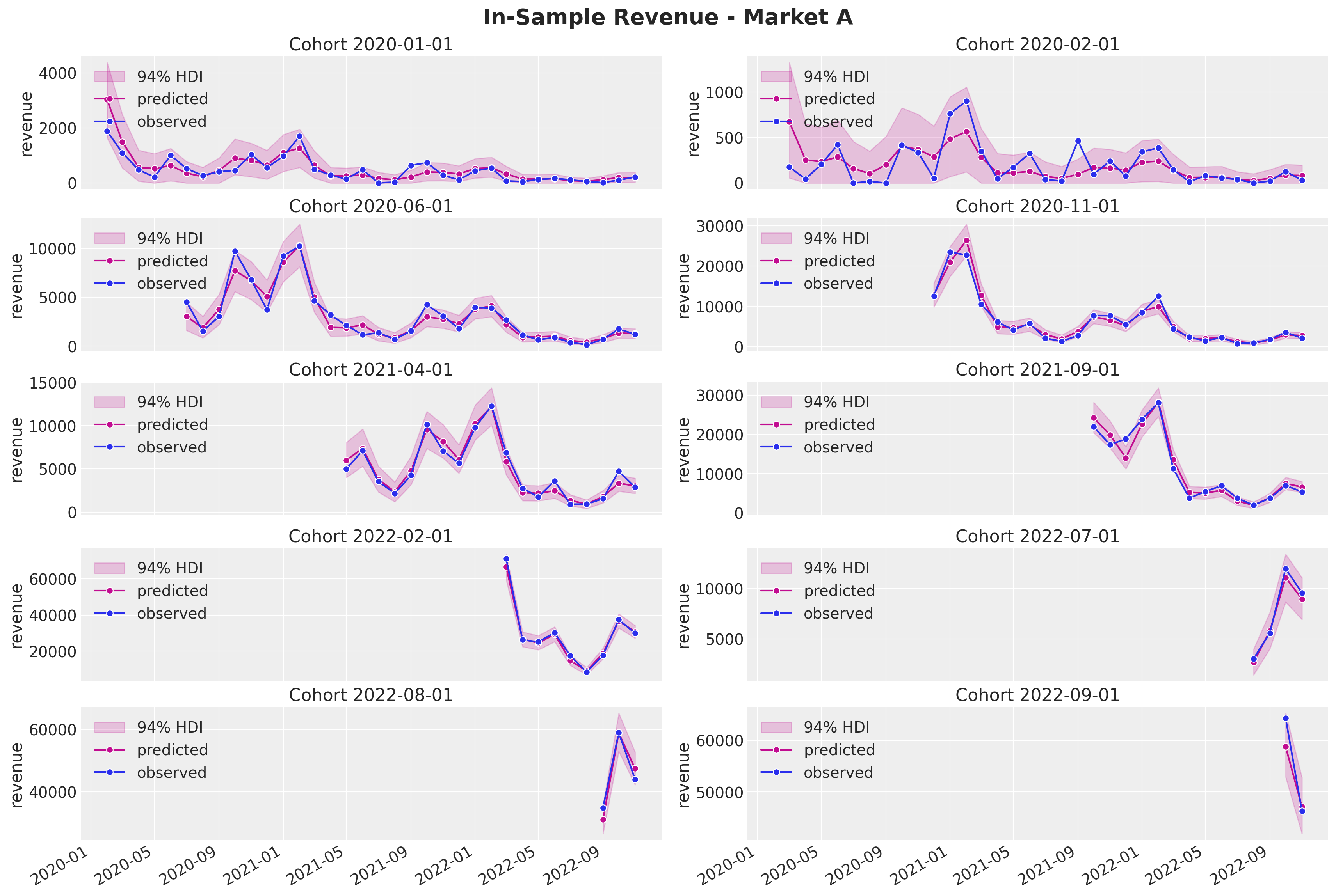
cohorts_to_plot = [
    datetime(2022, 3, 1, tzinfo=UTC),
    datetime(2022, 4, 1, tzinfo=UTC),
    datetime(2022, 5, 1, tzinfo=UTC),
    datetime(2022, 6, 1, tzinfo=UTC),
    datetime(2022, 7, 1, tzinfo=UTC),
    datetime(2022, 8, 1, tzinfo=UTC),
    datetime(2022, 9, 1, tzinfo=UTC),
    datetime(2022, 10, 1, tzinfo=UTC),
]

fig, axes = plt.subplots(
    nrows=np.ceil(len(cohorts_to_plot) / 2).astype(int),
    ncols=2,
    figsize=(17, 11),
    sharex=True,
    sharey=False,
    layout="constrained",
)

for cohort, ax in zip(cohorts_to_plot, axes.flatten(), strict=True):
    plot_train_revenue_hdi_cohort(market="B", cohort=cohort, ax=ax)

fig.suptitle("In-Sample Revenue - Market B", y=1.03, fontsize=20, fontweight="bold")
fig.autofmt_xdate()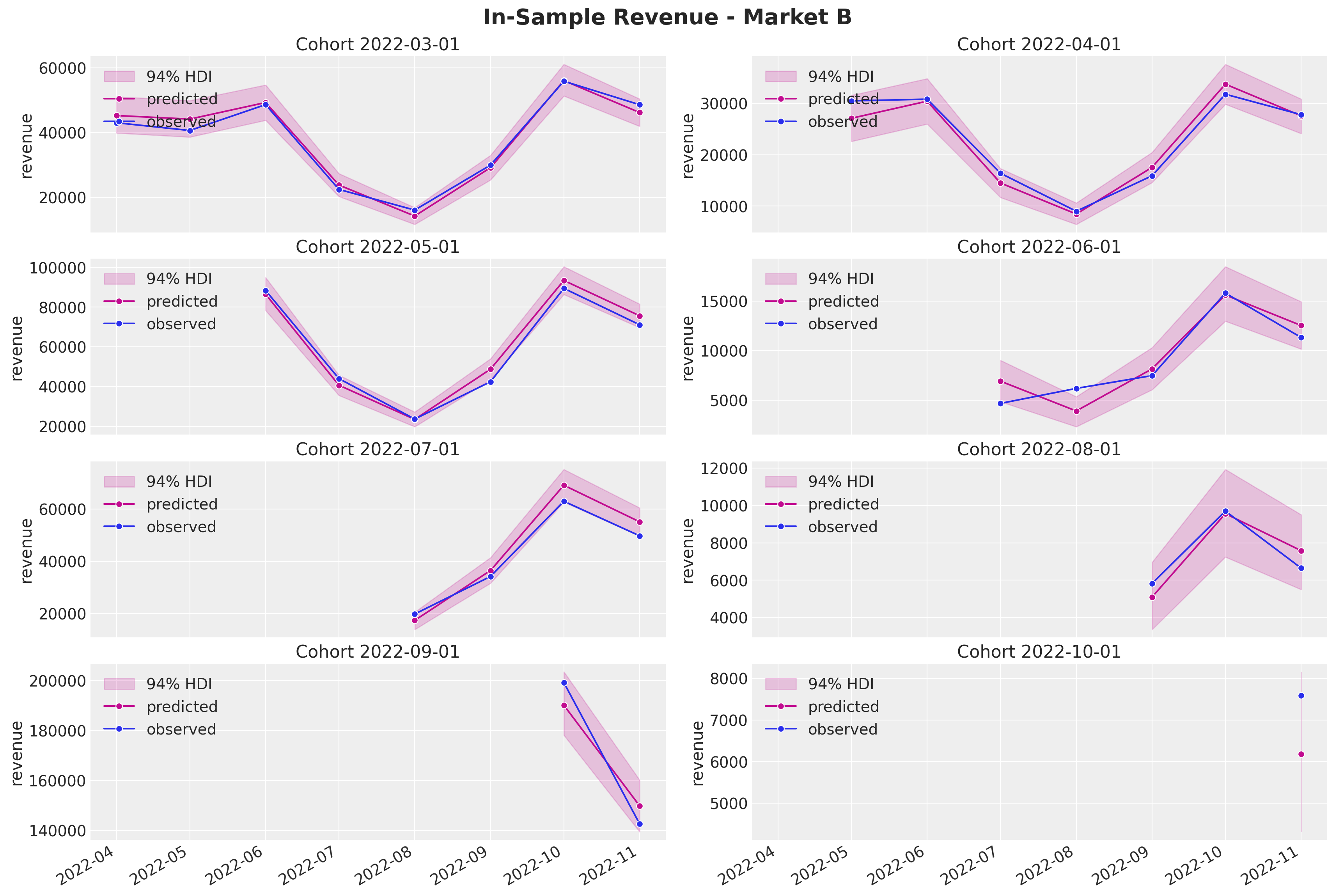
cohorts_to_plot = [
    datetime(2022, 3, 1, tzinfo=UTC),
    datetime(2022, 4, 1, tzinfo=UTC),
    datetime(2022, 5, 1, tzinfo=UTC),
    datetime(2022, 6, 1, tzinfo=UTC),
    datetime(2022, 7, 1, tzinfo=UTC),
    datetime(2022, 8, 1, tzinfo=UTC),
    datetime(2022, 9, 1, tzinfo=UTC),
    datetime(2022, 10, 1, tzinfo=UTC),
]

fig, axes = plt.subplots(
    nrows=np.ceil(len(cohorts_to_plot) / 2).astype(int),
    ncols=2,
    figsize=(17, 11),
    sharex=True,
    sharey=False,
    layout="constrained",
)

for cohort, ax in zip(cohorts_to_plot, axes.flatten(), strict=True):
    plot_train_revenue_hdi_cohort(market="C", cohort=cohort, ax=ax)

fig.suptitle("In-Sample Revenue - Market C", y=1.03, fontsize=20, fontweight="bold")
fig.autofmt_xdate()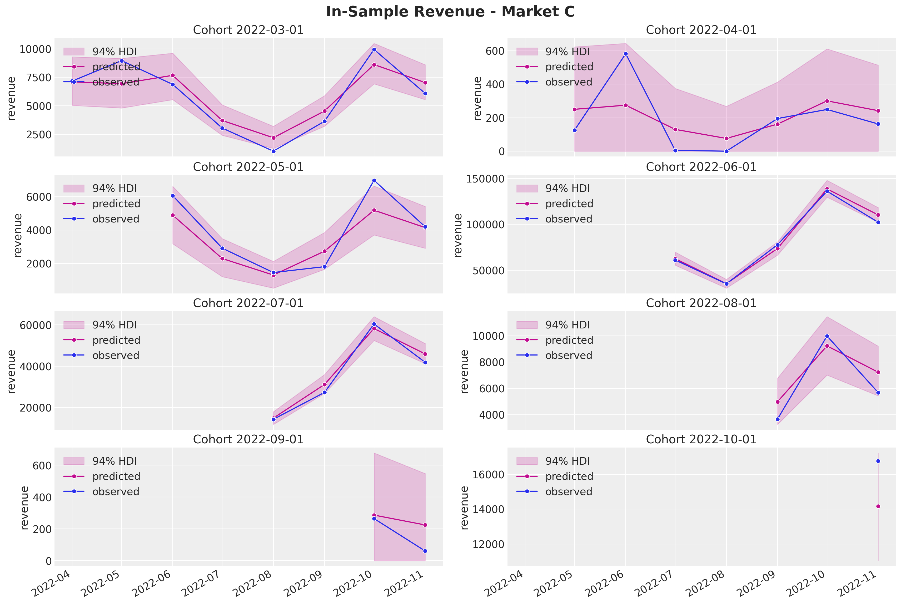
cohorts_to_plot = [
    datetime(2022, 7, 1, tzinfo=UTC),
    datetime(2022, 8, 1, tzinfo=UTC),
    datetime(2022, 9, 1, tzinfo=UTC),
    datetime(2022, 10, 1, tzinfo=UTC),
]

fig, axes = plt.subplots(
    nrows=np.ceil(len(cohorts_to_plot) / 2).astype(int),
    ncols=2,
    figsize=(17, 9),
    sharex=True,
    sharey=False,
    layout="constrained",
)

for cohort, ax in zip(cohorts_to_plot, axes.flatten(), strict=True):
    plot_train_revenue_hdi_cohort(market="D", cohort=cohort, ax=ax)

fig.suptitle("In-Sample Revenue - Market D", y=1.03, fontsize=20, fontweight="bold")
fig.autofmt_xdate()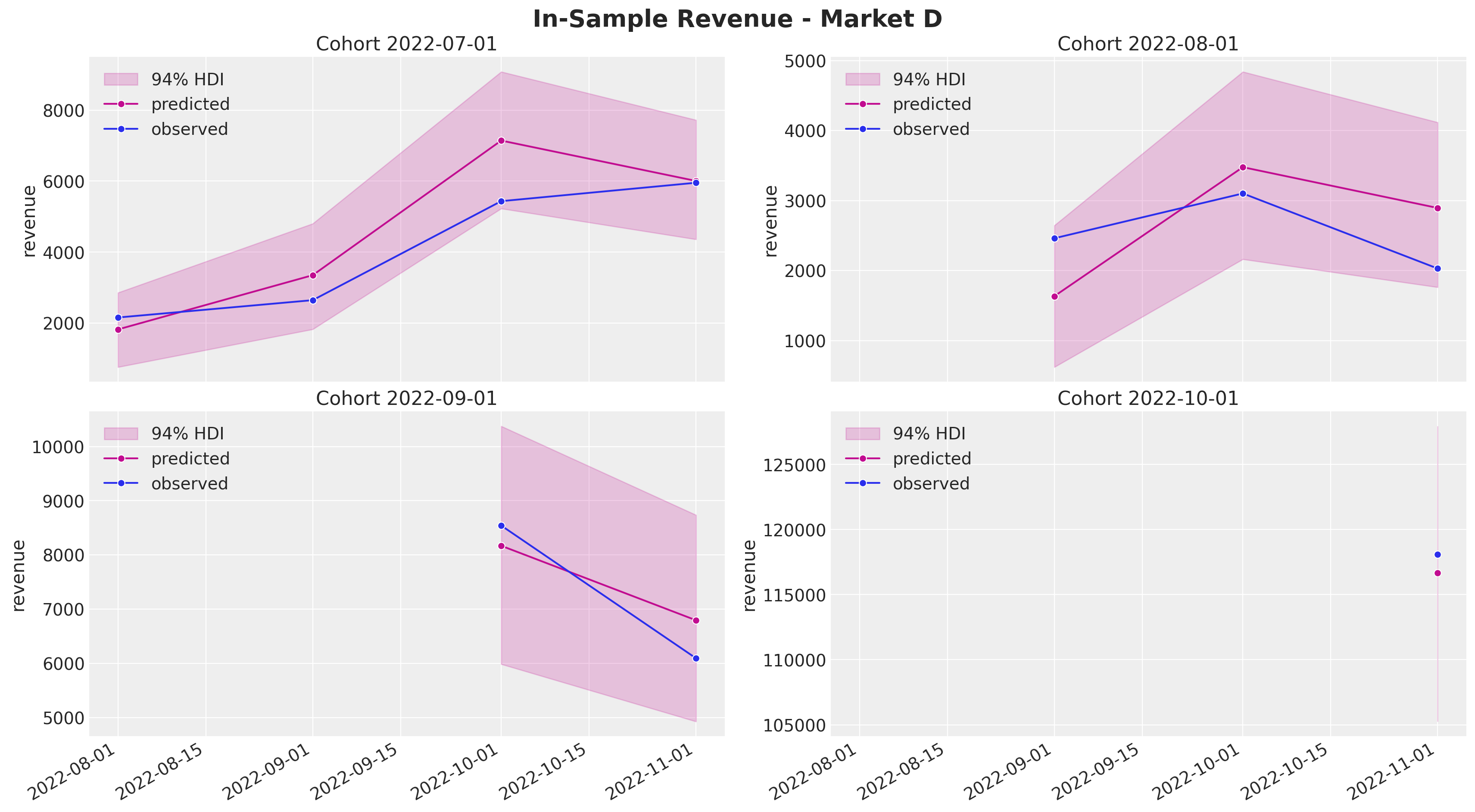
Again, the results look quite reasonable (not perfect though).
Out-of-Sample Predictions
Next, we focus on the out-of-sample performance of the model.
Data Preparation
It is very important to ensure the data is in the format expected by the model. We process the test set data with the transformers fitted on the training set.
test_data_red_df = test_data_df.filter(pl.col("cohort_age").gt(pl.lit(0)))
test_data_red_df = test_data_red_df.filter(
    pl.col("cohort").is_in(set(train_data_red_df["cohort"]))
)
test_obs_idx = jnp.array(range(test_data_red_df.shape[0]))
test_n_users = test_data_red_df["n_users"].to_jax()
test_n_active_users = test_data_red_df["n_active_users"].to_jax()
test_retention = test_data_red_df["retention"].to_jax()
test_revenue = test_data_red_df["revenue"].to_jax()

test_cohort = test_data_red_df["cohort"].to_numpy()
test_cohort_idx = train_cohort_encoder.transform(test_cohort).flatten()
test_period = test_data_red_df["period"].to_numpy()
test_market = test_data_red_df["market"].to_numpy()
test_market_idx = jnp.array(train_market_encoder.transform(test_market).flatten())

x_test = test_data_red_df[features]
x_test_preprocessed = preprocessor.transform(x_test)
x_test_preprocessed_array = jnp.array(x_test_preprocessed)

test_age = test_data_red_df["age"].to_numpy()
test_age_scaled = jnp.array(
    train_age_scaler.transform(test_age.reshape(-1, 1)).flatten()
)
test_cohort_age = test_data_red_df["cohort_age"].to_numpy()
test_cohort_age_scaled = jnp.array(
    train_cohort_age_scaler.transform(test_cohort_age.reshape(-1, 1)).flatten()
)
We proceed to make predictions on the test set.
test_predictive = Predictive(
    model=model, guide=guide, params=params, num_samples=4 * 2_000
)
rng_key, rng_subkey = random.split(key=rng_key)
test_posterior_predictive_samples = test_predictive(
    rng_subkey,
    x_test_preprocessed_array,
    test_age_scaled,
    test_cohort_age_scaled,
    test_n_users,
    test_market_idx,
)
test_idata = az.from_dict(
posterior_predictive={
k: np.expand_dims(a=np.asarray(v), axis=0)
for k, v in test_posterior_predictive_samples.items()
},
coords={"obs_idx": test_obs_idx},
dims={
"retention": ["obs_idx"],
"n_active_users": ["obs_idx"],
"revenue": ["obs_idx"],
"retention_estimated": ["obs_idx"],
},
)Now we are ready to asses the model performance.
Retention
We proceed very similar as above with the retention component.
test_retention_estimated_hdi = az.hdi(ary=test_idata["posterior_predictive"])[
    "retention_estimated"
]


def plot_test_retention_hdi_cohort(
    market: str, cohort: datetime, ax: plt.Axes
) -> plt.Axes:
    market_index = train_market_encoder.transform([market])[0]
    cohort_index = train_cohort_encoder.transform([cohort.replace(tzinfo=None)])[0]

    mask = (test_cohort_idx == cohort_index) & (
        np.array(test_market_idx) == market_index
    )

    test_period_range = test_data_red_df.filter(
        pl.col("cohort").eq(train_cohort_encoder.classes_[cohort_index])
        & pl.col("market").eq(train_market_encoder.classes_[market_index])
    )["period"].to_numpy()

    ax.fill_between(
        x=test_period_range,
        y1=test_retention_estimated_hdi[mask, :][:, 0],
        y2=test_retention_estimated_hdi[mask, :][:, 1],
        alpha=0.2,
        color="C2",
    )

    sns.lineplot(
        x=test_period_range,
        y=test_idata["posterior_predictive"]["retention_estimated"].mean(
            dim=["chain", "draw"]
        )[mask],
        marker="o",
        color="C2",
        ax=ax,
    )
    sns.lineplot(
        x=test_period_range,
        y=test_retention[mask],
        color="C0",
        marker="o",
        ax=ax,
    )
    return ax
cohorts_to_plot = [
datetime(2020, 1, 1, tzinfo=UTC),
datetime(2020, 2, 1, tzinfo=UTC),
datetime(2020, 6, 1, tzinfo=UTC),
datetime(2020, 11, 1, tzinfo=UTC),
datetime(2021, 4, 1, tzinfo=UTC),
datetime(2021, 9, 1, tzinfo=UTC),
datetime(2022, 2, 1, tzinfo=UTC),
datetime(2022, 7, 1, tzinfo=UTC),
datetime(2022, 8, 1, tzinfo=UTC),
datetime(2022, 9, 1, tzinfo=UTC),
]
fig, axes = plt.subplots(
nrows=len(cohorts_to_plot),
ncols=1,
figsize=(15, 18),
sharex=True,
sharey=True,
layout="constrained",
)
for cohort, ax in zip(cohorts_to_plot, axes.flatten(), strict=True):
plot_train_retention_hdi_cohort(market="A", cohort=cohort, ax=ax)
plot_test_retention_hdi_cohort(market="A", cohort=cohort, ax=ax)
ax.axvline(
x=period_train_test_split,
color="black",
linestyle="--",
label="train/test split",
)
ax.legend(loc="center left", bbox_to_anchor=(1, 0.5))
fig.suptitle("Retention Predictions - Market A", y=1.03, fontsize=20, fontweight="bold")
fig.autofmt_xdate()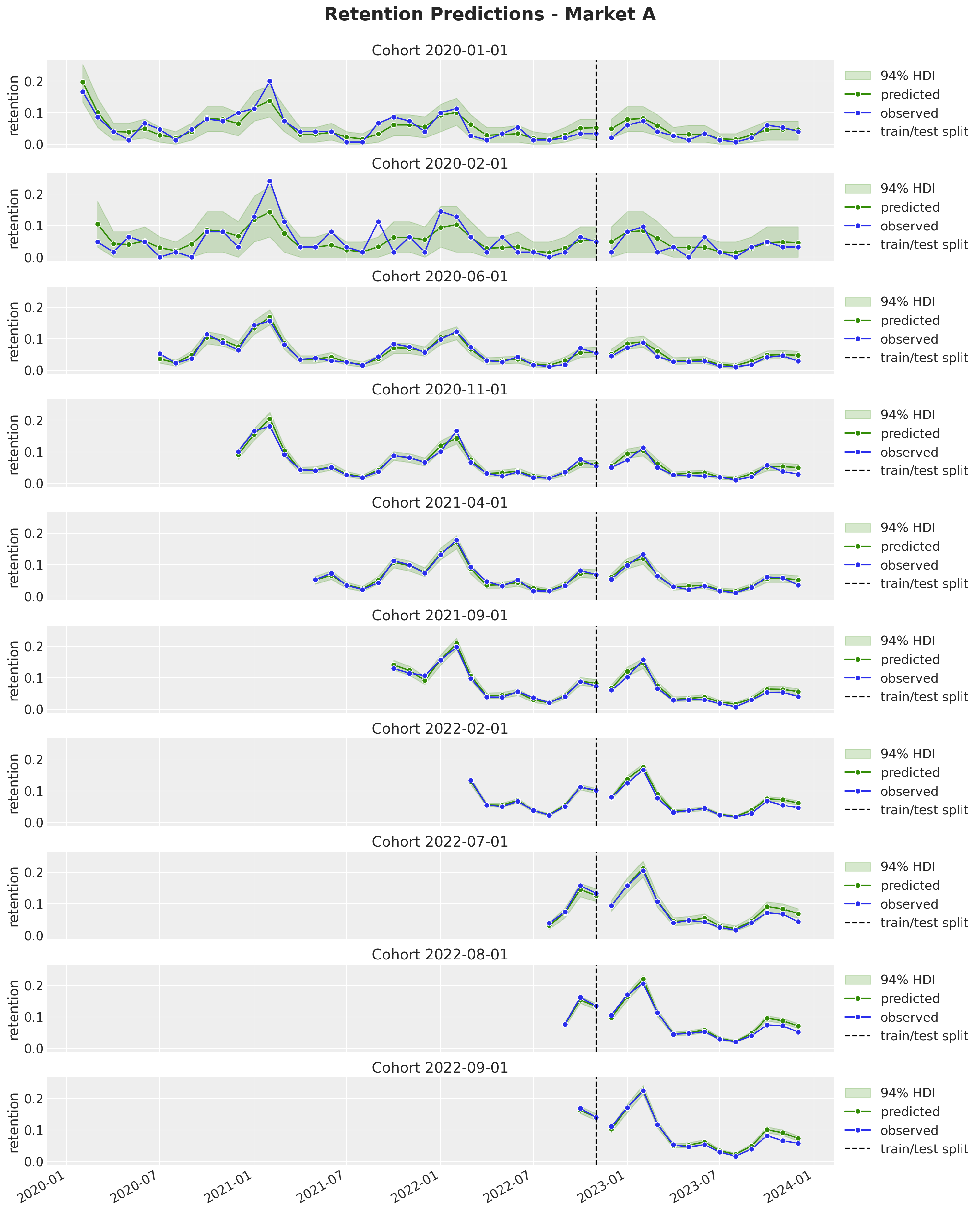
cohorts_to_plot = [
    datetime(2022, 3, 1, tzinfo=UTC),
    datetime(2022, 4, 1, tzinfo=UTC),
    datetime(2022, 5, 1, tzinfo=UTC),
    datetime(2022, 6, 1, tzinfo=UTC),
    datetime(2022, 7, 1, tzinfo=UTC),
    datetime(2022, 8, 1, tzinfo=UTC),
    datetime(2022, 9, 1, tzinfo=UTC),
    datetime(2022, 10, 1, tzinfo=UTC),
]

fig, axes = plt.subplots(
    nrows=len(cohorts_to_plot),
    ncols=1,
    figsize=(15, 15),
    sharex=True,
    sharey=True,
    layout="constrained",
)

for cohort, ax in zip(cohorts_to_plot, axes.flatten(), strict=True):
    plot_train_retention_hdi_cohort(market="B", cohort=cohort, ax=ax)
    plot_test_retention_hdi_cohort(market="B", cohort=cohort, ax=ax)
    ax.axvline(
        x=period_train_test_split,
        color="black",
        linestyle="--",
        label="train/test split",
    )
    ax.legend(loc="center left", bbox_to_anchor=(1, 0.5))

fig.suptitle("Retention Predictions - Market B", y=1.03, fontsize=20, fontweight="bold")
fig.autofmt_xdate()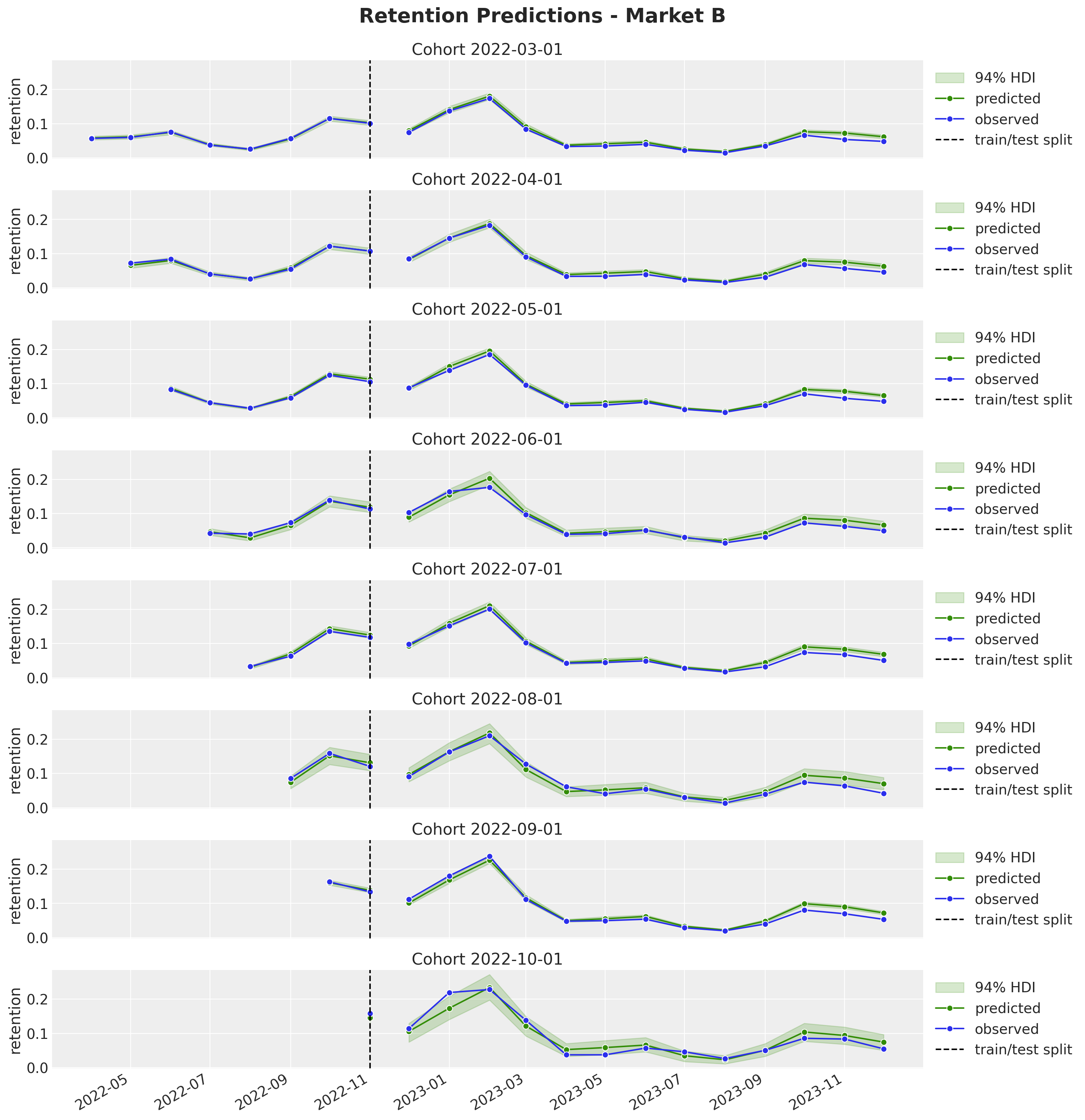
cohorts_to_plot = [
    datetime(2022, 3, 1, tzinfo=UTC),
    datetime(2022, 4, 1, tzinfo=UTC),
    datetime(2022, 5, 1, tzinfo=UTC),
    datetime(2022, 6, 1, tzinfo=UTC),
    datetime(2022, 7, 1, tzinfo=UTC),
    datetime(2022, 8, 1, tzinfo=UTC),
    datetime(2022, 9, 1, tzinfo=UTC),
    datetime(2022, 10, 1, tzinfo=UTC),
]

fig, axes = plt.subplots(
    nrows=len(cohorts_to_plot),
    ncols=1,
    figsize=(15, 15),
    sharex=True,
    sharey=True,
    layout="constrained",
)

for cohort, ax in zip(cohorts_to_plot, axes.flatten(), strict=True):
    plot_train_retention_hdi_cohort(market="C", cohort=cohort, ax=ax)
    plot_test_retention_hdi_cohort(market="C", cohort=cohort, ax=ax)
    ax.axvline(
        x=period_train_test_split,
        color="black",
        linestyle="--",
        label="train/test split",
    )
    ax.legend(loc="center left", bbox_to_anchor=(1, 0.5))

fig.suptitle("Retention Predictions - Market C", y=1.03, fontsize=20, fontweight="bold")
fig.autofmt_xdate()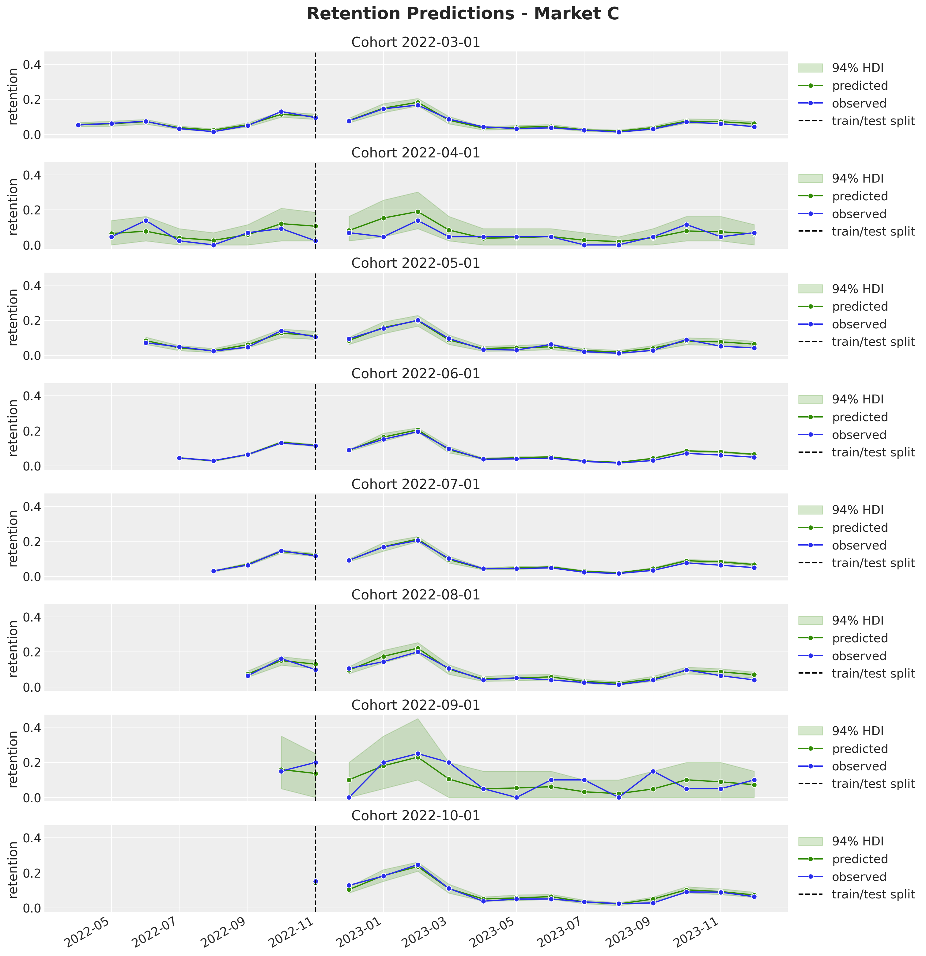
cohorts_to_plot = [
    datetime(2022, 7, 1, tzinfo=UTC),
    datetime(2022, 8, 1, tzinfo=UTC),
    datetime(2022, 9, 1, tzinfo=UTC),
    datetime(2022, 10, 1, tzinfo=UTC),
]

fig, axes = plt.subplots(
    nrows=len(cohorts_to_plot),
    ncols=1,
    figsize=(15, 9),
    sharex=True,
    sharey=True,
    layout="constrained",
)

for cohort, ax in zip(cohorts_to_plot, axes.flatten(), strict=True):
    plot_train_retention_hdi_cohort(market="D", cohort=cohort, ax=ax)
    plot_test_retention_hdi_cohort(market="D", cohort=cohort, ax=ax)
    ax.axvline(
        x=period_train_test_split,
        color="black",
        linestyle="--",
        label="train/test split",
    )
    ax.legend(loc="center left", bbox_to_anchor=(1, 0.5))

fig.suptitle("Retention Predictions - Market D", y=1.03, fontsize=20, fontweight="bold")
fig.autofmt_xdate()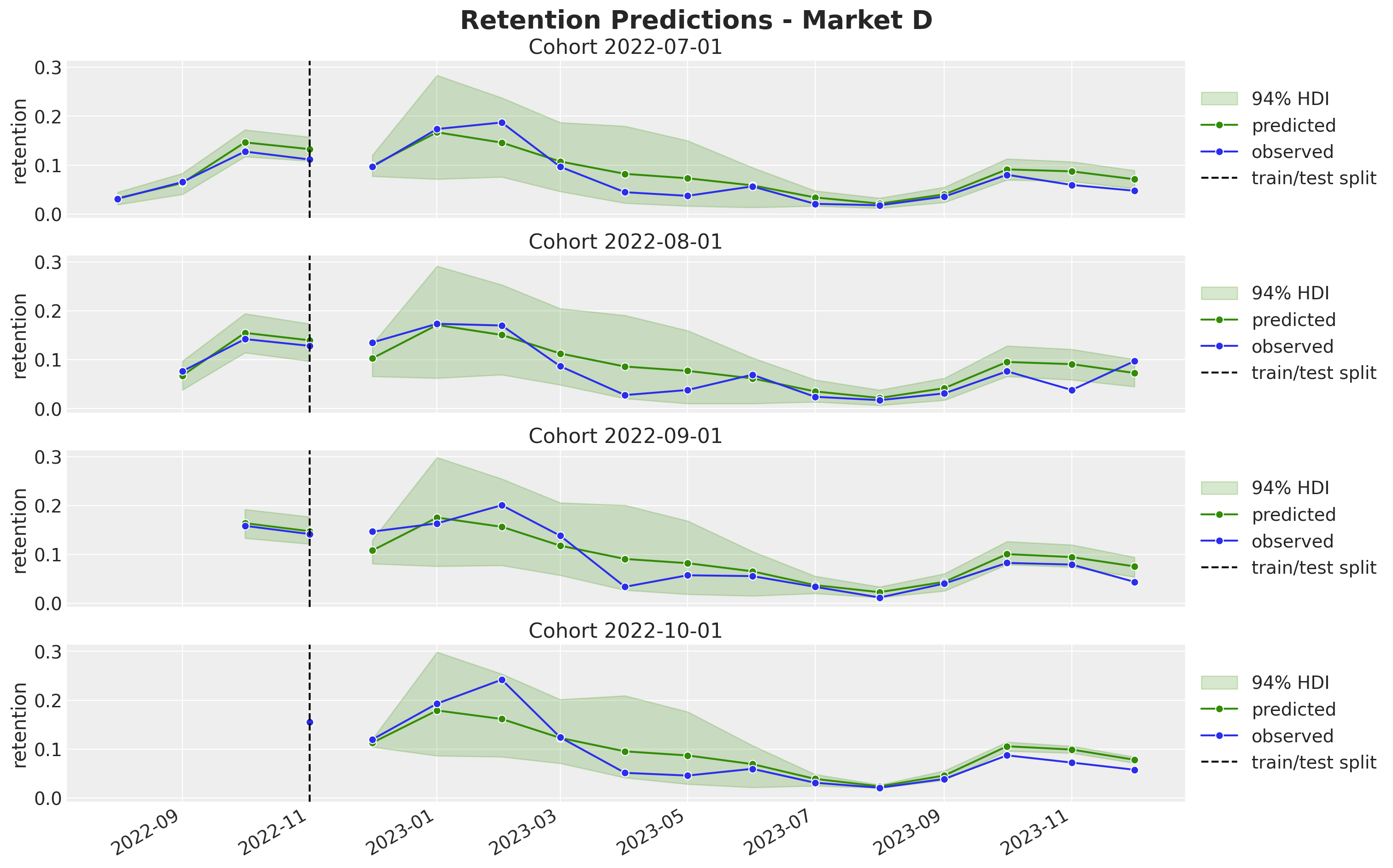
All the out-of-sample predictions look quite reasonable. Here are some important observations:
It seems the model is overestimating the retention for the later periods (it’s still a one-year horizon).
We are able to generate very reasonable predictions for market \(D\) where we have very few cohorts. Note that we even captured the yearly seasonality. This would have been impossible to do with a model trained on each market separately.
Revenue
We continue with the revenue component.
test_revenue_hdi = az.hdi(ary=test_idata["posterior_predictive"])["revenue"]


def plot_test_revenue_hdi_cohort(
    market: str, cohort: datetime, ax: plt.Axes
) -> plt.Axes:
    market_index = train_market_encoder.transform([market])[0]
    cohort_index = train_cohort_encoder.transform([cohort.replace(tzinfo=None)])[0]

    mask = (test_cohort_idx == cohort_index) & (
        np.array(test_market_idx) == market_index
    )

    test_period_range = test_data_red_df.filter(
        pl.col("cohort").eq(train_cohort_encoder.classes_[cohort_index])
        & pl.col("market").eq(train_market_encoder.classes_[market_index])
    )["period"].to_numpy()

    ax.fill_between(
        x=test_period_range,
        y1=test_revenue_hdi[mask, :][:, 0],
        y2=test_revenue_hdi[mask, :][:, 1],
        alpha=0.2,
        color="C3",
    )

    sns.lineplot(
        x=test_period_range,
        y=test_idata["posterior_predictive"]["revenue"].mean(dim=["chain", "draw"])[
            mask
        ],
        marker="o",
        color="C3",
        ax=ax,
    )
    sns.lineplot(
        x=test_period_range,
        y=test_revenue[mask],
        color="C0",
        marker="o",
        ax=ax,
    )
    return ax
cohorts_to_plot = [
datetime(2020, 1, 1, tzinfo=UTC),
datetime(2020, 2, 1, tzinfo=UTC),
datetime(2020, 6, 1, tzinfo=UTC),
datetime(2020, 11, 1, tzinfo=UTC),
datetime(2021, 4, 1, tzinfo=UTC),
datetime(2021, 9, 1, tzinfo=UTC),
datetime(2022, 2, 1, tzinfo=UTC),
datetime(2022, 7, 1, tzinfo=UTC),
datetime(2022, 8, 1, tzinfo=UTC),
datetime(2022, 9, 1, tzinfo=UTC),
]
fig, axes = plt.subplots(
nrows=len(cohorts_to_plot),
ncols=1,
figsize=(15, 18),
sharex=True,
sharey=False,
layout="constrained",
)
for cohort, ax in zip(cohorts_to_plot, axes.flatten(), strict=True):
plot_train_revenue_hdi_cohort(market="A", cohort=cohort, ax=ax)
plot_test_revenue_hdi_cohort(market="A", cohort=cohort, ax=ax)
ax.axvline(
x=period_train_test_split,
color="black",
linestyle="--",
label="train/test split",
)
ax.legend(loc="center left", bbox_to_anchor=(1, 0.5))
fig.suptitle("Revenue Predictions - Market A", y=1.03, fontsize=20, fontweight="bold")
fig.autofmt_xdate()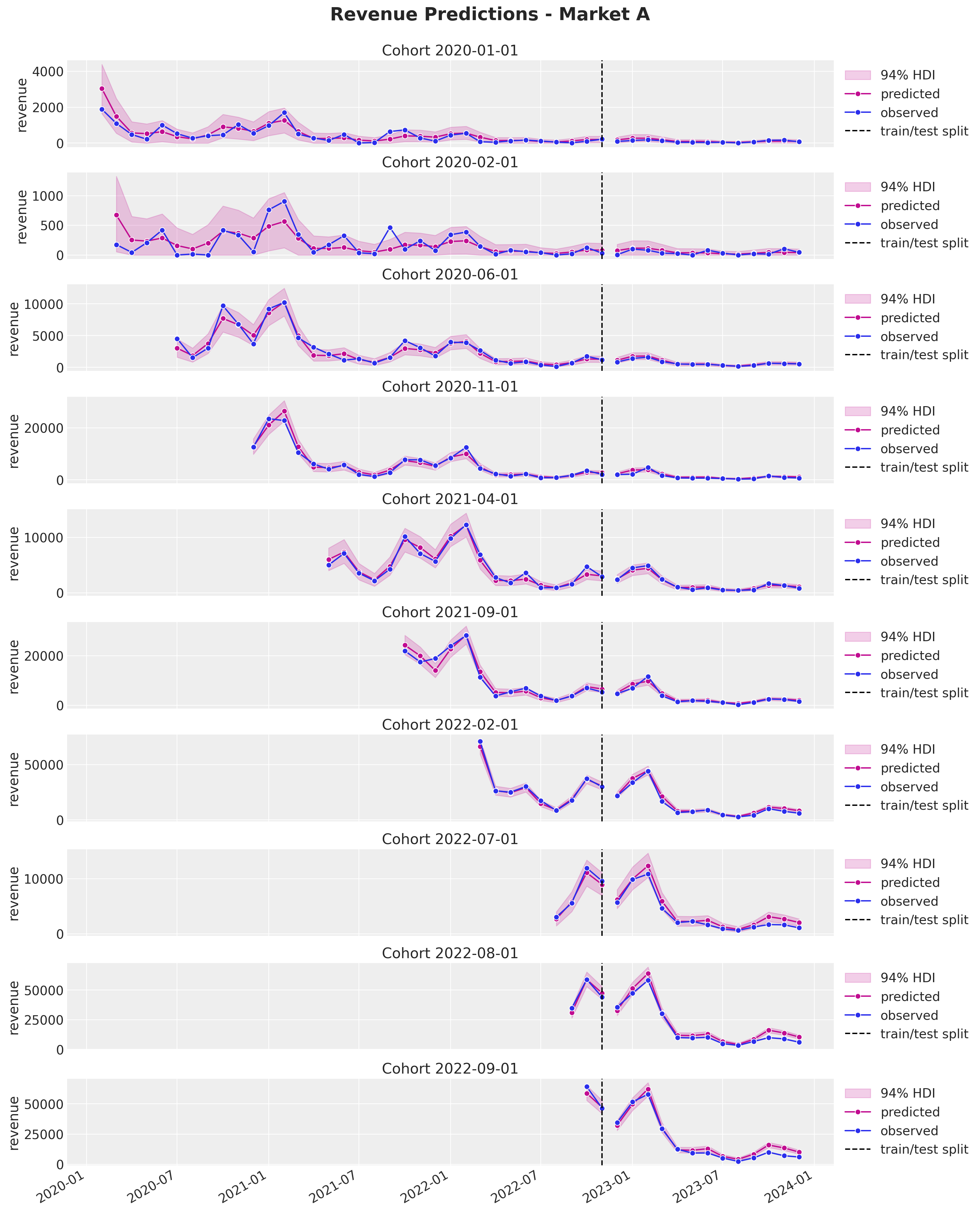
cohorts_to_plot = [
    datetime(2022, 3, 1, tzinfo=UTC),
    datetime(2022, 4, 1, tzinfo=UTC),
    datetime(2022, 5, 1, tzinfo=UTC),
    datetime(2022, 6, 1, tzinfo=UTC),
    datetime(2022, 7, 1, tzinfo=UTC),
    datetime(2022, 8, 1, tzinfo=UTC),
    datetime(2022, 9, 1, tzinfo=UTC),
    datetime(2022, 10, 1, tzinfo=UTC),
]

fig, axes = plt.subplots(
    nrows=len(cohorts_to_plot),
    ncols=1,
    figsize=(15, 15),
    sharex=True,
    sharey=False,
    layout="constrained",
)

for cohort, ax in zip(cohorts_to_plot, axes.flatten(), strict=True):
    plot_train_revenue_hdi_cohort(market="B", cohort=cohort, ax=ax)
    plot_test_revenue_hdi_cohort(market="B", cohort=cohort, ax=ax)
    ax.axvline(
        x=period_train_test_split,
        color="black",
        linestyle="--",
        label="train/test split",
    )
    ax.legend(loc="center left", bbox_to_anchor=(1, 0.5))

fig.suptitle("Revenue Predictions - Market B", y=1.03, fontsize=20, fontweight="bold")
fig.autofmt_xdate()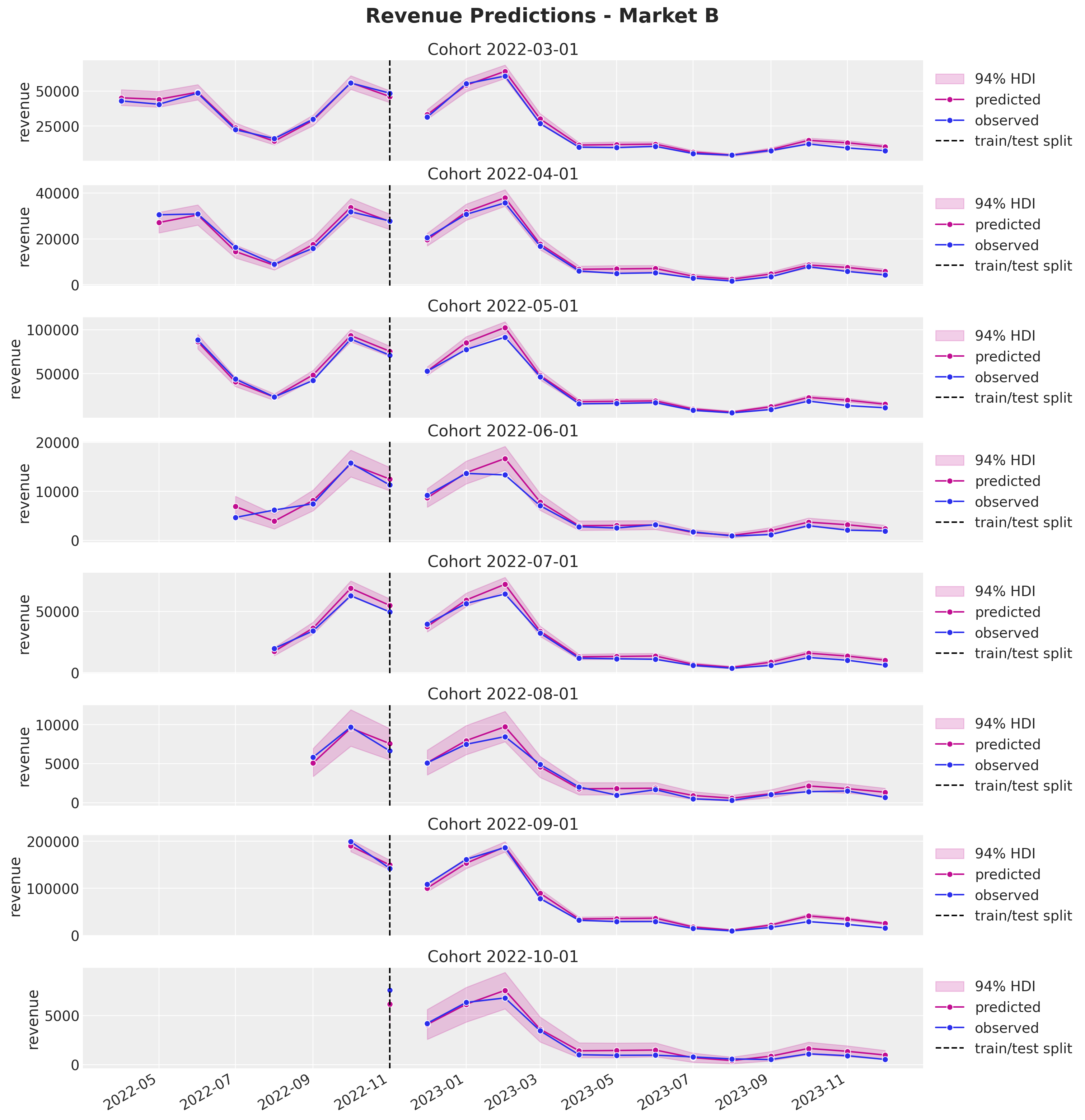
cohorts_to_plot = [
    datetime(2022, 3, 1, tzinfo=UTC),
    datetime(2022, 4, 1, tzinfo=UTC),
    datetime(2022, 5, 1, tzinfo=UTC),
    datetime(2022, 6, 1, tzinfo=UTC),
    datetime(2022, 7, 1, tzinfo=UTC),
    datetime(2022, 8, 1, tzinfo=UTC),
    datetime(2022, 9, 1, tzinfo=UTC),
    datetime(2022, 10, 1, tzinfo=UTC),
]

fig, axes = plt.subplots(
    nrows=len(cohorts_to_plot),
    ncols=1,
    figsize=(15, 15),
    sharex=True,
    sharey=False,
    layout="constrained",
)

for cohort, ax in zip(cohorts_to_plot, axes.flatten(), strict=True):
    plot_train_revenue_hdi_cohort(market="C", cohort=cohort, ax=ax)
    plot_test_revenue_hdi_cohort(market="C", cohort=cohort, ax=ax)
    ax.axvline(
        x=period_train_test_split,
        color="black",
        linestyle="--",
        label="train/test split",
    )
    ax.legend(loc="center left", bbox_to_anchor=(1, 0.5))

fig.suptitle("Revenue Predictions - Market C", y=1.03, fontsize=20, fontweight="bold")
fig.autofmt_xdate()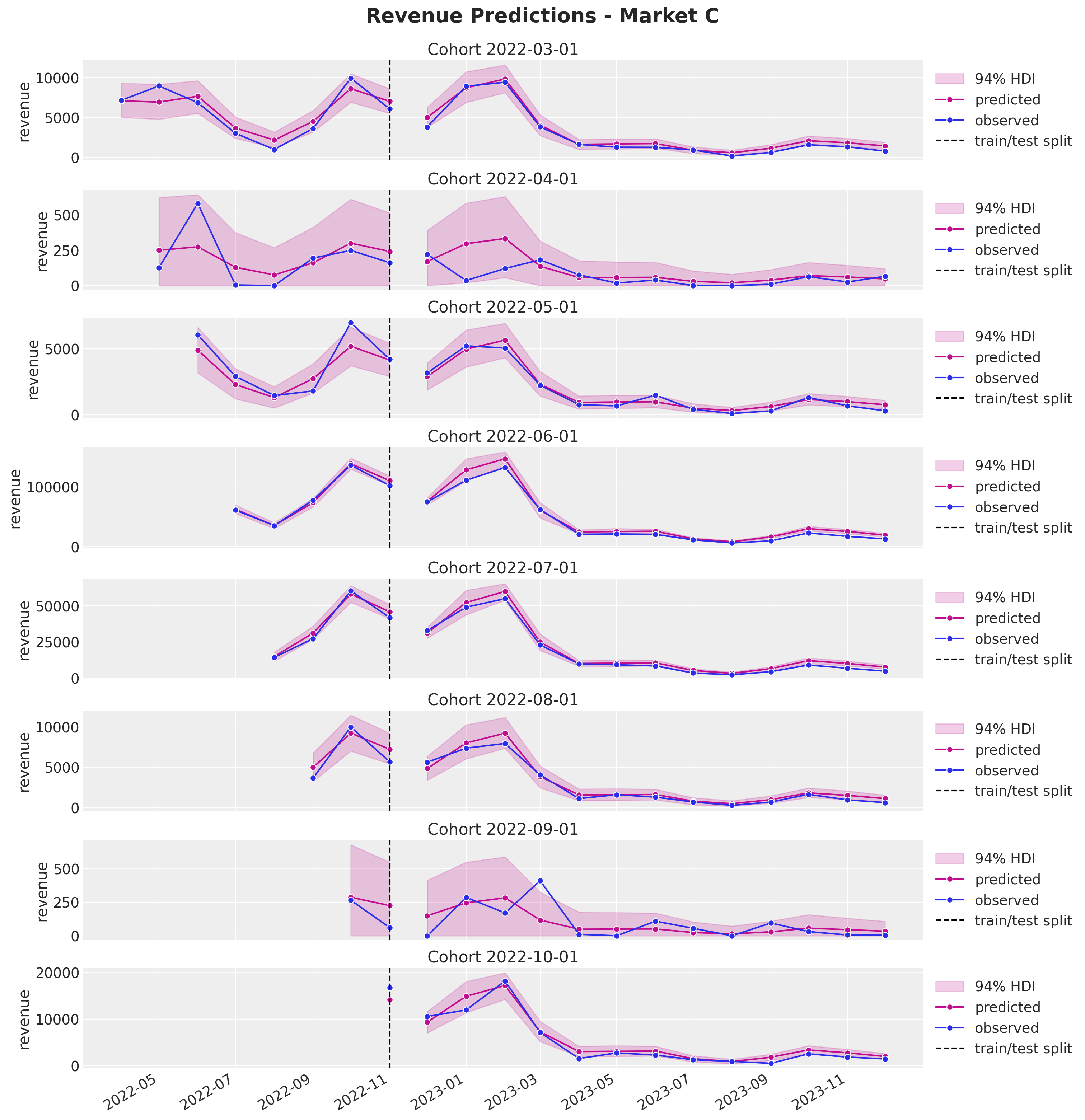
cohorts_to_plot = [
    datetime(2022, 7, 1, tzinfo=UTC),
    datetime(2022, 8, 1, tzinfo=UTC),
    datetime(2022, 9, 1, tzinfo=UTC),
    datetime(2022, 10, 1, tzinfo=UTC),
]

fig, axes = plt.subplots(
    nrows=len(cohorts_to_plot),
    ncols=1,
    figsize=(15, 10),
    sharex=True,
    sharey=False,
    layout="constrained",
)

for cohort, ax in zip(cohorts_to_plot, axes.flatten(), strict=True):
    plot_train_revenue_hdi_cohort(market="D", cohort=cohort, ax=ax)
    plot_test_revenue_hdi_cohort(market="D", cohort=cohort, ax=ax)
    ax.axvline(
        x=period_train_test_split,
        color="black",
        linestyle="--",
        label="train/test split",
    )
    ax.legend(loc="center left", bbox_to_anchor=(1, 0.5))

fig.suptitle("Revenue Predictions - Market D", y=1.03, fontsize=20, fontweight="bold")
fig.autofmt_xdate()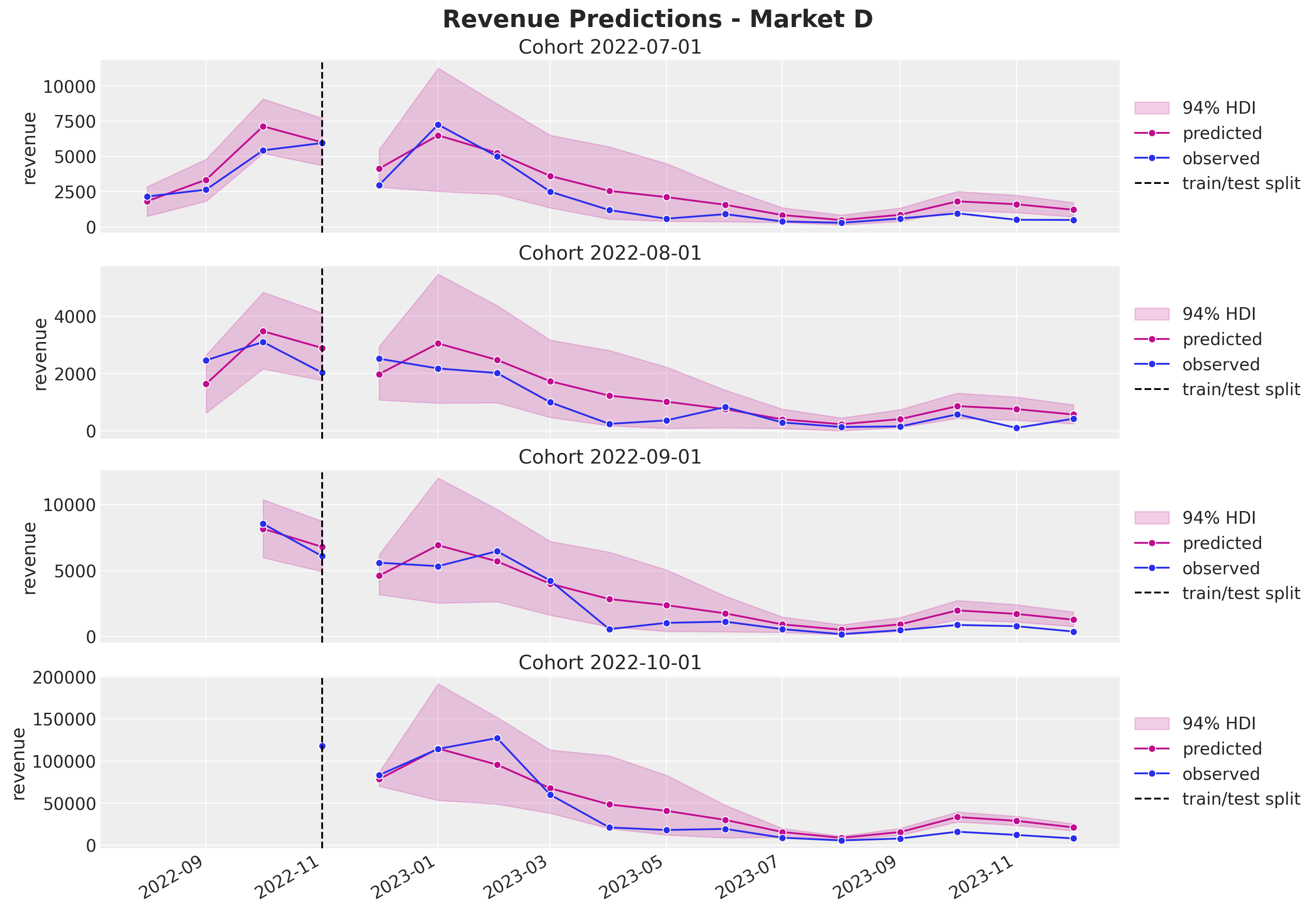
Again, the predictions look, in general, quite good. In particular observe from the last plot how much we can capture out of market D. This illustrates the power of the approach. On the other hand, we keep seeing a mild overestimation for the later periods.
Aggregated Predictions
Finally, let’s show how to visualize the aggregated predictions.
train_total_revenue_predicted = (
    idata["posterior_predictive"]["revenue"]
    .rename({"obs_idx": "period_month"})
    .assign_coords(period_month=train_period)
    .groupby("period_month")
    .sum()
)

test_total_revenue_predicted = (
    test_idata["posterior_predictive"]["revenue"]
    .rename({"obs_idx": "period_month"})
    .assign_coords(period_month=test_period)
    .groupby("period_month")
    .sum()
)


fig, ax = plt.subplots()

az.plot_hdi(
    x=train_total_revenue_predicted.coords["period_month"],
    y=train_total_revenue_predicted,
    hdi_prob=0.94,
    color="C0",
    smooth=False,
    fill_kwargs={"alpha": 0.7, "label": "$94\\%$ HDI (train)"},
    ax=ax,
)

az.plot_hdi(
    x=test_total_revenue_predicted.coords["period_month"],
    y=test_total_revenue_predicted,
    hdi_prob=0.94,
    color="C1",
    smooth=False,
    fill_kwargs={"alpha": 0.7, "label": "$94\\%$ HDI (est)"},
    ax=ax,
)

(
    data_df.filter(pl.col("cohort_age").gt(pl.lit(0)))
    .filter(pl.col("cohort").is_in(set(train_data_red_df["cohort"])))
    .group_by("period")
    .agg(pl.col("revenue").sum())
    .pipe(
        sns.lineplot,
        x="period",
        y="revenue",
        color="black",
        marker="o",
        ax=ax,
    )
)

ax.axvline(
    x=period_train_test_split,
    color="gray",
    linestyle="--",
    label="train/test split",
)

ax.legend(loc="upper left")

ax.set_title("Total Revenue", fontsize=18, fontweight="bold");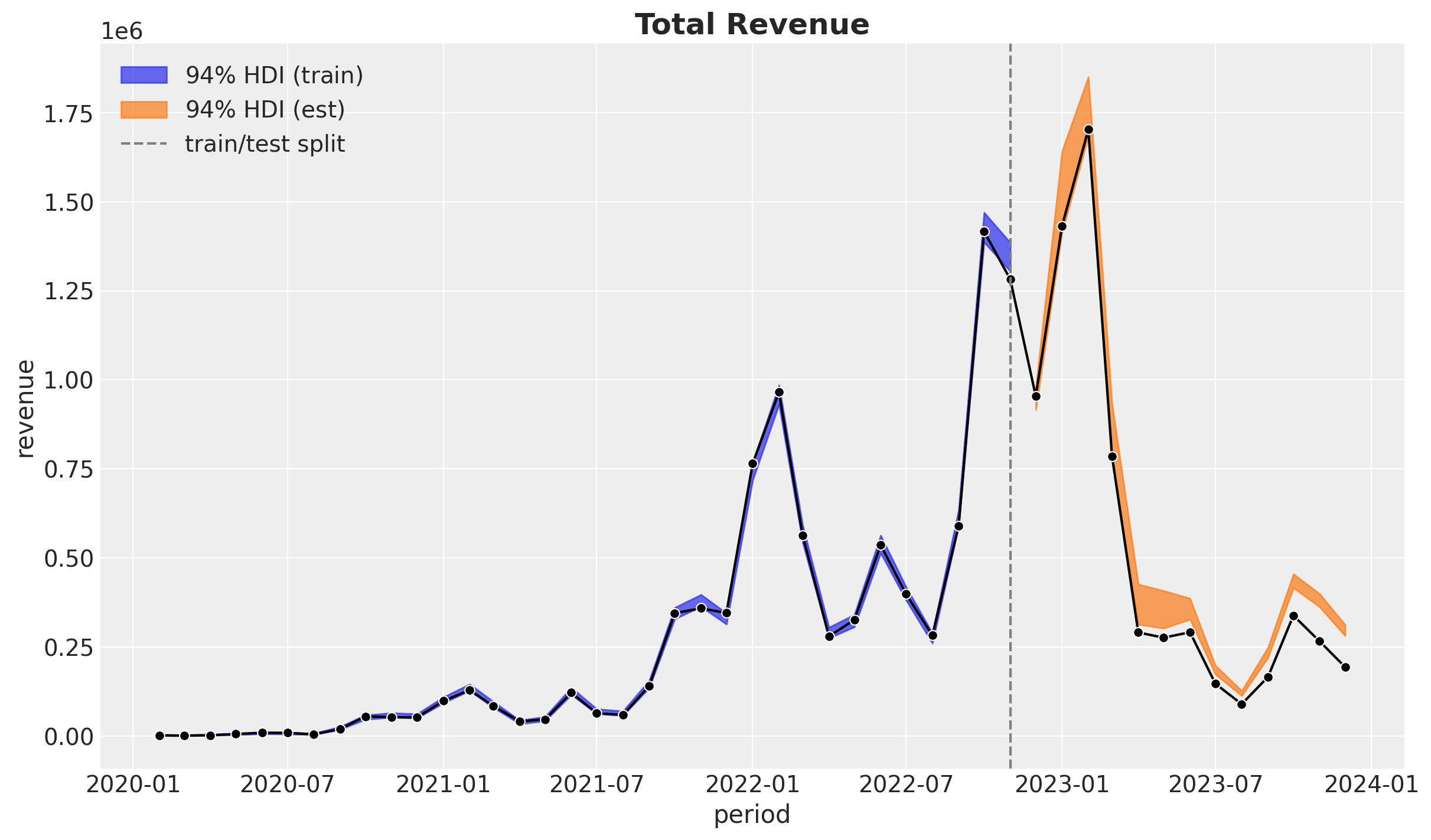
This last plot shows the aggregated predictions for the revenue (removing cohort age equal to \(0\)). Overall the fit and predictions are good. Still, we can see that the model is overestimating the revenue for the later periods as expected from the previous sections.
Now let’s look into the market split.
fig, axes = plt.subplots(
    nrows=len(markets),
    ncols=1,
    figsize=(15, 15),
    sharex=True,
    sharey=True,
    layout="constrained",
)

axes = axes.flatten()

for market, ax in zip(markets, axes, strict=True):
    train_total_revenue_predicted = (
        idata["posterior_predictive"]["revenue"]
        .rename({"obs_idx": "market"})
        .assign_coords(market=train_market)
        .sel(market=market.name)
        .rename({"market": "period_month"})
        .assign_coords(period_month=train_period[train_market == market.name])
        .groupby("period_month")
        .sum()
    )

    test_total_revenue_predicted = (
        test_idata["posterior_predictive"]["revenue"]
        .rename({"obs_idx": "market"})
        .assign_coords(market=test_market)
        .sel(market=market.name)
        .rename({"market": "period_month"})
        .assign_coords(period_month=test_period[test_market == market.name])
        .groupby("period_month")
        .sum()
    )

    az.plot_hdi(
        x=train_total_revenue_predicted.coords["period_month"],
        y=train_total_revenue_predicted,
        hdi_prob=0.94,
        color="C0",
        smooth=False,
        fill_kwargs={"alpha": 0.7, "label": "$94\\%$ HDI (train)"},
        ax=ax,
    )

    az.plot_hdi(
        x=test_total_revenue_predicted.coords["period_month"],
        y=test_total_revenue_predicted,
        hdi_prob=0.94,
        color="C1",
        smooth=False,
        fill_kwargs={"alpha": 0.7, "label": "$94\\%$ HDI (est)"},
        ax=ax,
    )

    (
        data_df.filter(
            pl.col("cohort_age").gt(pl.lit(0))
            & pl.col("market").eq(pl.lit(market.name))
            & pl.col("cohort").is_in(set(train_data_red_df["cohort"]))
        )
        .group_by("period")
        .agg(pl.col("revenue").sum())
        .pipe(
            sns.lineplot,
            x="period",
            y="revenue",
            color="black",
            marker="o",
            ax=ax,
        )
    )

    ax.axvline(
        x=period_train_test_split,
        color="gray",
        linestyle="--",
        label="train/test split",
    )

    ax.legend(loc="upper left")

    ax.set_title(
        f"Total Revenue - Market {market.name}", fontsize=18, fontweight="bold"
    )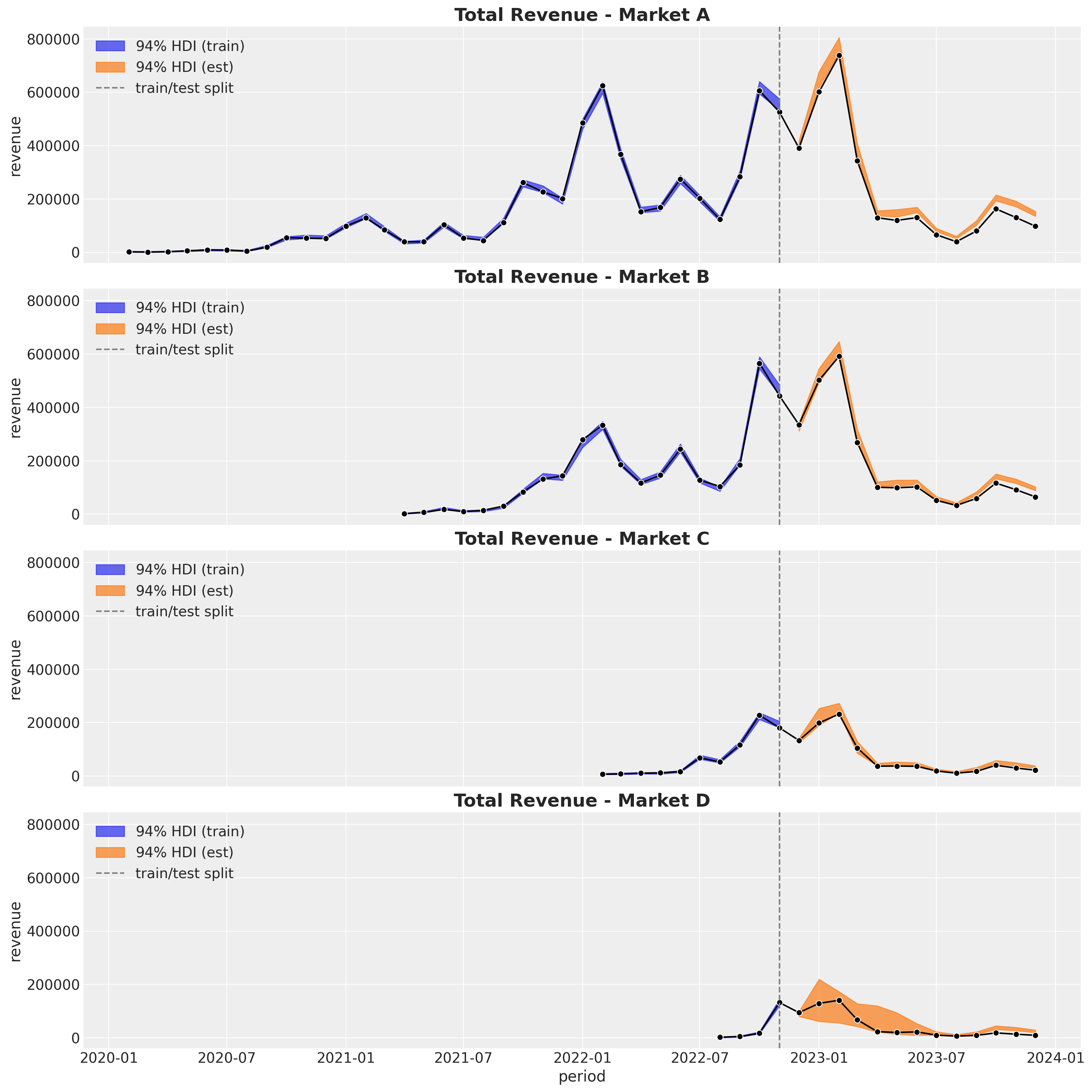
Interestingly, it seems the over-estimation is coming from the more mature markets.
Summary
This notebook successfully demonstrates the extension of cohort revenue and retention modeling to a hierarchical framework across multiple markets. The key contributions and findings include:
Model Architecture:
- Combined a neural network for retention modeling with a hierarchical linear model for revenue prediction.
- Used Stochastic Variational Inference (SVI) for scalable parameter estimation across markets.
- Implemented market-specific parameters with shared hierarchical priors to enable information pooling.
Key Benefits:
- Information Sharing: Markets with limited data (like Market \(D\) with only \(4\) cohorts) benefit from information borrowed from more mature markets.
- Seasonal Pattern Capture: Successfully captured yearly seasonality patterns even in data-sparse markets.
- Scalability: SVI approach enables scaling to tens or hundreds of markets.
Results:
- Strong in-sample fit for both retention and revenue components across all markets.
- Reasonable out-of-sample predictions with proper uncertainty quantification.
- Demonstrated ability to forecast for young markets that would be impossible to model individually.
- Identified systematic overestimation in later periods, particularly from mature markets.
The hierarchical approach proves particularly valuable for businesses operating across multiple markets with varying maturity levels, enabling better forecasting and decision-making through principled uncertainty quantification and information sharing.