In this notebook we present an example of how to use a combination of Bayesian hierarchical models and the non-parametric methods , namely bayesian additive trees (BART), to model the product life cycles. This approach is motivated by previous work in cohort analysis, see here.
As a case study we use the Google search index (trends) data for iPhones worldwide. We use the data of four different models to predict the development of the latest iPhone. The model presented for this specific example can be easily extended for other products and product life cycles structures.
Prepare Notebook
import arviz as az
import holidays
import matplotlib.pyplot as plt
import numpy as np
import pandas as pd
import preliz as pz
import pymc as pm
import pymc_bart as pmb
import pytensor.tensor as pt
import seaborn as sns
from pymc_bart.split_rules import ContinuousSplitRule, OneHotSplitRule, SubsetSplitRule

az.style.use("arviz-darkgrid")
plt.rcParams["figure.figsize"] = [12, 7]
plt.rcParams["figure.dpi"] = 100
plt.rcParams["figure.facecolor"] = "white"

%load_ext autoreload
%autoreload 2
%config InlineBackend.figure_format = "retina"
seed: int = sum(map(ord, "iphone_trends"))
rng: np.random.Generator = np.random.default_rng(seed=seed)Read Data
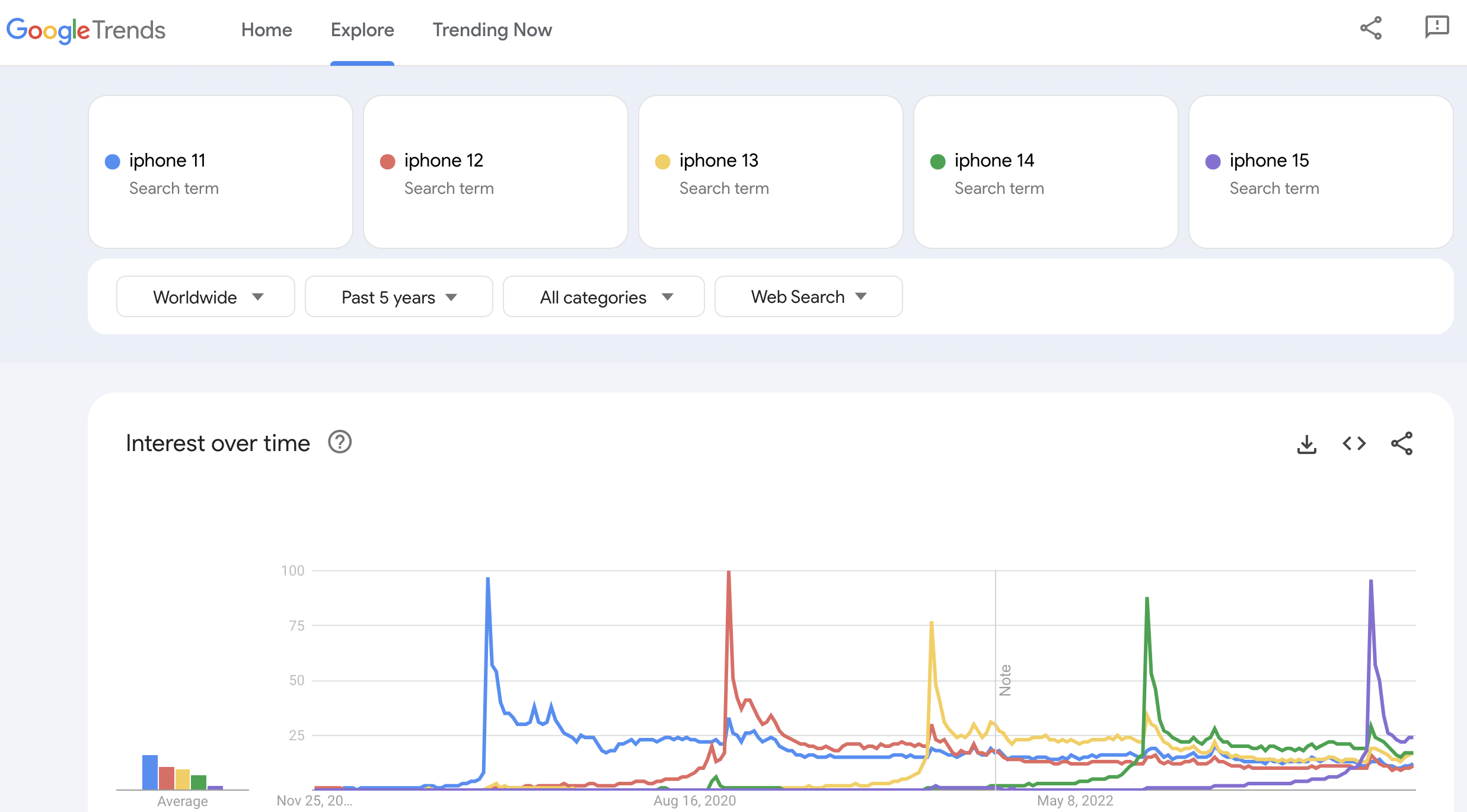
We provide the data downloaded from Google Trends for the following search terms (weekly granularity):
raw_df = pd.read_csv(
    "https://raw.githubusercontent.com/juanitorduz/website_projects/master/data/iphone_trends.csv",
    parse_dates=["week"]
)

raw_df.tail()| week | iphone_11 | iphone_12 | iphone_13 | iphone_14 | iphone_15 | |
|---|---|---|---|---|---|---|
| 256 | 2023-10-22 | 10 | 10 | 14 | 16 | 23 |
| 257 | 2023-10-29 | 10 | 9 | 13 | 15 | 22 |
| 258 | 2023-11-05 | 11 | 10 | 15 | 17 | 22 |
| 259 | 2023-11-12 | 11 | 10 | 16 | 17 | 24 |
| 260 | 2023-11-19 | 12 | 11 | 17 | 17 | 24 |
We see a clear structure in the searches development for each model:
- Steep peak at the beginning of the product life cycle (maximum on the release week)
- A slow long term decay with a mild yearly seasonality.
In order to capture the peak at the beginning of the product life cycle we collect the release data for such iPhone models:
releases_df = pd.DataFrame(
    data=[
        {"model": "iphone_11", "release_date": "September 20, 2019"},
        {"model": "iphone_12", "release_date": "October 23, 2020"},
        {"model": "iphone_13", "release_date": "September 24, 2021"},
        {"model": "iphone_14", "release_date": "September 16, 2022"},
        {"model": "iphone_15", "release_date": "September 22, 2023"},
    ]
)

# We use the same week-starting date as the Google Trends data
release_dates_df = releases_df.assign(
    release_week=lambda x: (
        pd.to_datetime(x["release_date"]).dt.to_period("W-SAT").dt.start_time
        - pd.DateOffset(days=7)
    )
)

release_dates_df.head()| model | release_date | release_week | |
|---|---|---|---|
| 0 | iphone_11 | September 20, 2019 | 2019-09-08 |
| 1 | iphone_12 | October 23, 2020 | 2020-10-11 |
| 2 | iphone_13 | September 24, 2021 | 2021-09-12 |
| 3 | iphone_14 | September 16, 2022 | 2022-09-04 |
| 4 | iphone_15 | September 22, 2023 | 2023-09-10 |
Feature Engineering
To start, we collect two holiday events that are clear from the image above: Black Friday and Christmas.
holidays_list = ["Christmas Day", "Thanksgiving"]

holidays_df = (
    pd.DataFrame.from_dict(
        data=holidays.country_holidays(
            country="US", years=[2019, 2020, 2021, 2022, 2023, 2024]
        ),
        orient="index",
        columns=["holiday"],
    )
    .query("holiday in @holidays_list")
    .reset_index(drop=False)
    .rename(columns={"index": "date"})
    .assign(
        week=lambda x: pd.to_datetime(x["date"]).dt.to_period("W-SAT").dt.start_time
    )
)

holidays_df.head(12)| date | holiday | week | |
|---|---|---|---|
| 0 | 2019-11-28 | Thanksgiving | 2019-11-24 |
| 1 | 2019-12-25 | Christmas Day | 2019-12-22 |
| 2 | 2020-11-26 | Thanksgiving | 2020-11-22 |
| 3 | 2020-12-25 | Christmas Day | 2020-12-20 |
| 4 | 2021-11-25 | Thanksgiving | 2021-11-21 |
| 5 | 2021-12-25 | Christmas Day | 2021-12-19 |
| 6 | 2022-11-24 | Thanksgiving | 2022-11-20 |
| 7 | 2022-12-25 | Christmas Day | 2022-12-25 |
| 8 | 2023-11-23 | Thanksgiving | 2023-11-19 |
| 9 | 2023-12-25 | Christmas Day | 2023-12-24 |
| 10 | 2024-11-28 | Thanksgiving | 2024-11-24 |
| 11 | 2024-12-25 | Christmas Day | 2024-12-22 |
Next, motivated by the features used in the previous work on cohort analysis, we create the following features:
age: Number of weeks since the release of the iPhone model relative to today’s date.model_age: Number of weeks since the release of the iPhone model relative to the release of the latest iPhone model. Not that this feature is negative for weeks before the release.is_release_week: Binary feature indicating if the week is the release week of the iPhone model.month: Month of the year.
data_df = (
    raw_df.copy()
    .melt(id_vars=["week"], var_name="model", value_name="search")
    .merge(right=release_dates_df, on="model")
    .drop(columns=["release_date"])
    .assign(
        age=lambda x: (x["week"].max() - x["week"]).dt.days / 7,
        model_age=lambda x: (x["week"] - x["release_week"]).dt.days / 7,
        is_release=lambda x: (x["model_age"] == 0).astype(float),
        month=lambda x: x["week"].dt.month,
        # holidays
        is_christmas=lambda x: x["week"]
        .isin(holidays_df.query("holiday == 'Christmas Day'")["week"])
        .astype(float),
        is_thanksgiving=lambda x: x["week"]
        .isin(holidays_df.query("holiday == 'Thanksgiving'")["week"])
        .astype(float),
    )
    .query(
        "model_age >= -50"
    )  # Drop data one year before release (as it is mainly noise)
    .reset_index(drop=True)
)

data_df.head()| week | model | search | release_week | age | model_age | is_release | month | is_christmas | is_thanksgiving | |
|---|---|---|---|---|---|---|---|---|---|---|
| 0 | 2018-11-25 | iphone_11 | 0 | 2019-09-08 | 260.0 | -41.0 | 0.0 | 11 | 0.0 | 0.0 |
| 1 | 2018-12-02 | iphone_11 | 0 | 2019-09-08 | 259.0 | -40.0 | 0.0 | 12 | 0.0 | 0.0 |
| 2 | 2018-12-09 | iphone_11 | 0 | 2019-09-08 | 258.0 | -39.0 | 0.0 | 12 | 0.0 | 0.0 |
| 3 | 2018-12-16 | iphone_11 | 0 | 2019-09-08 | 257.0 | -38.0 | 0.0 | 12 | 0.0 | 0.0 |
| 4 | 2018-12-23 | iphone_11 | 0 | 2019-09-08 | 256.0 | -37.0 | 0.0 | 12 | 0.0 | 0.0 |
EDA
We plot the data for each iPhone model:
fig, ax = plt.subplots(figsize=(15, 7))

sns.lineplot(
    data=data_df,
    x="week",
    y="search",
    hue="model",
    ax=ax,
)

for i, model in enumerate(release_dates_df["model"]):
    release_week = release_dates_df.query(f"model == '{model}'")["release_week"].item()
    ax.axvline(
        release_week,
        color=f"C{i}",
        linestyle="--",
        alpha=0.5,
        label=f"release week {model}",
    )

ax.legend(bbox_to_anchor=(1.05, 1), loc="upper left")
ax.set_title(
    label="Google Trends for iPhone Models (Worldwide)", fontsize=18, fontweight="bold"
)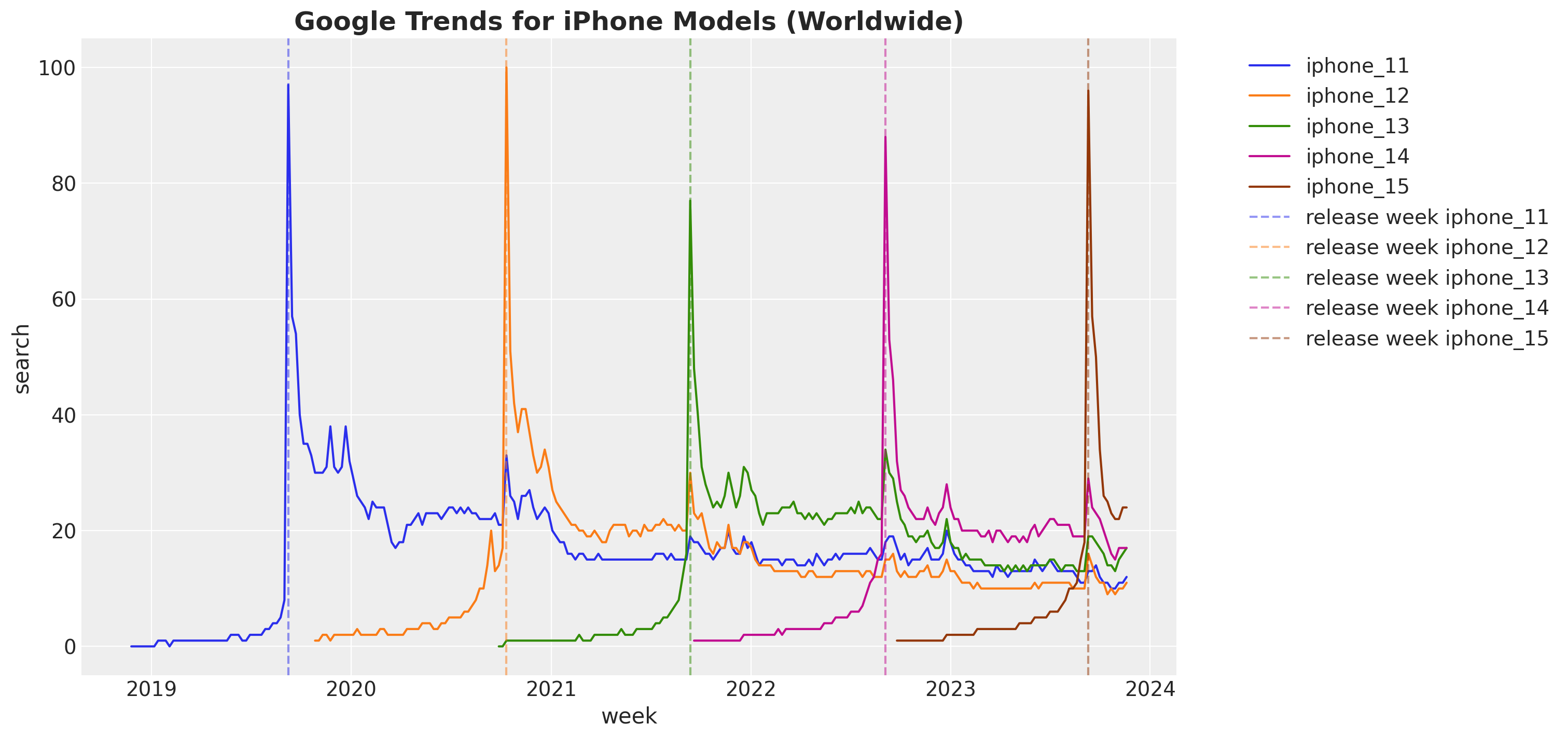
We do see how the peak maximum coincides with the release date.
Note that all of the models have a similar structure, however the maximum and decay forms differ from model to model. This motivates the use of a hierarchical model.
On the other hand, if we plot the search index in a heat map we doo see the immediate similarity to th cohort analysis problem where we use age and cohort age as key futures to model the revenue and retention:
fig, ax = plt.subplots()
(
    data_df.assign(week=lambda x: x["week"].dt.date)[["model", "week", "search"]]
    .pivot_table(index="model", columns="week", values="search")
    .pipe(
        (sns.heatmap, "data"),
        cmap="viridis_r",
        ax=ax,
    )
)
ax.set_title(
    label="Google Trends for iPhone Models (Worldwide)", fontsize=18, fontweight="bold"
)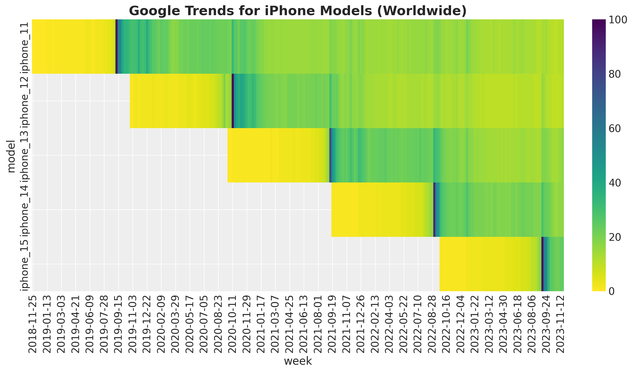
This motivates the use of BART as a non-parametric component to model seasonal and long term behavior of the search index.
Remark: This is of course not the only possibility. We could for example use (hierarchical) Gaussian processes.
Prepare Data
We now prepare the data for the model.
# model for the holdout data
test_model = "iphone_15"

train_df = data_df.query(f"model != '{test_model}'")
test_df = data_df.query(f"model == '{test_model}'")
train_obs = train_df.index.to_numpy()
train_iphone_model_idx, train_iphone_model = train_df["model"].factorize(sort=True)
train_month_idx, train_month = train_df["month"].factorize(sort=True)
train_age = train_df["age"].to_numpy()
train_model_age = train_df["model_age"].to_numpy()
train_is_release = train_df["is_release"].to_numpy()
features = ["age", "model_age", "month", "is_christmas", "is_thanksgiving"]
x_train = train_df[features]
train_search = train_df["search"].to_numpy()Model Specification
Main Idea
The main idea is to model the search index through a negative binomial likelihood where the mean is the sum of the release phase plus the long term decay. For the release phase we use a non-symmetric Gaussian bump function while for the long term decay we use a BART model.
Remark: We use the recommended parametrization for the negative binomial distribution, see here.
Remark: We weight the \(\alpha\) parameter in the likelihood to place more importance on the search index values closer to the release date. The motivation is that we are often interested in this first phase much more than the relatively stable decay (see here).
Mathematical Formulation
Here are the main ingredients of the model:
\[ \begin{align*} \beta^{[m]}_{\text{release}} \sim & \text{HalfNormal}(\sigma_{\beta}) \\ \ell^{[m]}_{\pm} \sim & \text{HalfNormal}(\sigma_{\ell}) \\ \mu_{\text{release}} = & \beta^{[m]}_{\text{release}} \left( I\{\text{model_age} \leq 0\} \exp(-{\text{model_age}^{p_{-}} / \ell^{[m]}_{-}}) \right. \\ & \left.+ I\{\text{model_age} \geq 0\} \exp(-{\text{model_age}^{p_{+}} / \ell^{[m]}_{+}} ) \right)\\ \mu_{\text{decay}} = & \text{BART}(\text{age}, \text{model_age}, \text{month}, \text{holidays}) \\ \mu = & \mu_{\text{release}} + \mu_{\text{decay}} \\ \alpha = & \frac{1}{\sqrt{\tilde{\alpha}}} \\ \alpha_{\text{weighted}} = & \frac{\alpha}{|\text{model_age}|} \\ \text{search} \sim & \text{NegativeBinomial}(\mu, \alpha_{\text{weighted}}) \end{align*} \]
The hierarchical structure is encoded in \(\beta{\text{release}}\) and the \(\ell_{\pm}\) which come from a common prior for each model respectively.
I believe this mathematical formulation is not very intuitive, so let’s go to the PyMC code:
# small number for numerical stability
eps = np.finfo(float).eps

coords = {"month": train_month, "feature": features}

with pm.Model(coords=coords) as model:
    # --- Data Containers ---

    model.add_coord(name="iphone_model", values=train_iphone_model, mutable=True)
    model.add_coord(name="obs", values=train_obs, mutable=True)
    iphone_model_idx_data = pm.MutableData(
        name="iphone_model_idx_data", value=train_iphone_model_idx, dims="obs"
    )
    model_age_data = pm.MutableData(
        name="model_age_data", value=train_model_age, dims="obs"
    )
    x_data = pm.MutableData(name="x_data", value=x_train, dims=("obs", "feature"))
    search_data = pm.MutableData(name="search_data", value=train_search, dims="obs")

    # --- Priors ---

    power_minus = pm.Beta(name="power_minus", alpha=5, beta=15)
    power_plus = pm.Beta(name="power_plus", alpha=5, beta=15)

    sigma_ell_is_release_minus = pm.Exponential(
        name="sigma_ell_is_release_minus", lam=1
    )
    sigma_ell_is_release_plus = pm.Exponential(
        name="sigma_ell_is_release_plus", lam=1 / 4
    )
    sigma_is_release = pm.Exponential(name="sigma_is_release", lam=1 / 100)

    ell_is_release_minus = pm.HalfNormal(
        name="ell_is_release_minus",
        sigma=sigma_ell_is_release_minus,
        dims="iphone_model",
    )

    ell_is_release_plus = pm.HalfNormal(
        name="ell_is_release_plus", sigma=sigma_ell_is_release_plus, dims="iphone_model"
    )

    beta_is_release = pm.HalfNormal(
        name="beta_is_release", sigma=sigma_is_release, dims="iphone_model"
    )

    inv_alpha_lam = pm.HalfNormal(name="inv_alpha_lam", sigma=500)

    inv_alpha = pm.Exponential(name="inv_alpha", lam=inv_alpha_lam, dims="iphone_model")

    bart_mu_log = pmb.BART(
        name="bart_mu_log",
        X=x_data,
        Y=np.log1p(train_search),
        m=100,
        response="mix",
        split_rules=[
            ContinuousSplitRule(),
            ContinuousSplitRule(),
            SubsetSplitRule(),
            OneHotSplitRule(),
            OneHotSplitRule(),
        ],
        dims="obs",
    )

    # --- Parametrization ---

    is_release_bump = pm.Deterministic(
        name="is_release_bump",
        var=beta_is_release[iphone_model_idx_data]
        * (
            (
                (model_age_data < 0)
                * pt.exp(
                    -pt.pow(pt.abs(model_age_data), power_minus)
                    / ell_is_release_minus[iphone_model_idx_data]
                )
            )
            + (
                (model_age_data >= 0)
                * pt.exp(
                    -pt.pow(pt.abs(model_age_data), power_plus)
                    / ell_is_release_plus[iphone_model_idx_data]
                )
            )
        ),
        dims="obs",
    )

    mu = pm.Deterministic(
        name="mu",
        var=pt.exp(bart_mu_log) + is_release_bump,
        dims="obs",
    )

    alpha = pm.Deterministic(
        name="alpha",
        var=1 / (pt.sqrt(inv_alpha) + eps),
        dims="iphone_model",
    )

    alpha_weighted = pm.Deterministic(
        name="alpha_weighted",
        var=alpha[iphone_model_idx_data] / (pt.abs(model_age_data) + 1),
        dims="obs",
    )

    # --- Likelihood ---

    _ = pm.NegativeBinomial(
        name="likelihood",
        mu=mu,
        alpha=alpha_weighted,
        observed=search_data,
        dims="obs",
    )

pm.model_to_graphviz(model=model)
We can take a look into some of the prior distributions for the Gaussian bump parameters:
fig, ax = plt.subplots(
    nrows=2, ncols=1, figsize=(9, 7), sharex=False, sharey=False, layout="constrained"
)
pz.Beta(alpha=5, beta=15).plot_pdf(ax=ax[0])
ax[0].set_title(r"$p_{\pm}$")
pz.Exponential(lam=1 / 4).plot_pdf(ax=ax[1])
ax[1].set_title(r"$\sigma_{\ell}$")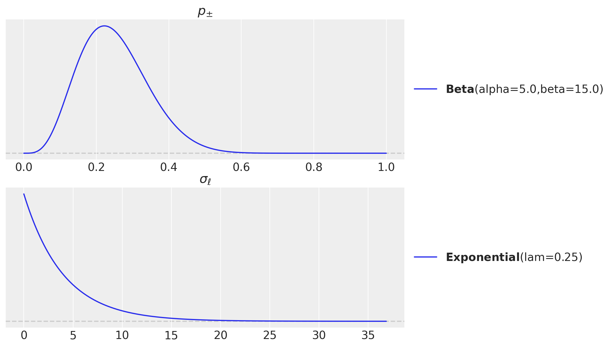
Prior Predictive
Let’s start with the prior predictive distribution to check the feasibility of the priors and the model specification:
with model:
    prior_predictive = pm.sample_prior_predictive(samples=1_000, random_seed=rng)
fig, ax = plt.subplots()
az.plot_ppc(data=prior_predictive, group="prior", kind="kde", ax=ax)
ax.set_title(label="Prior Predictive", fontsize=18, fontweight="bold")
ax.set(xscale="log")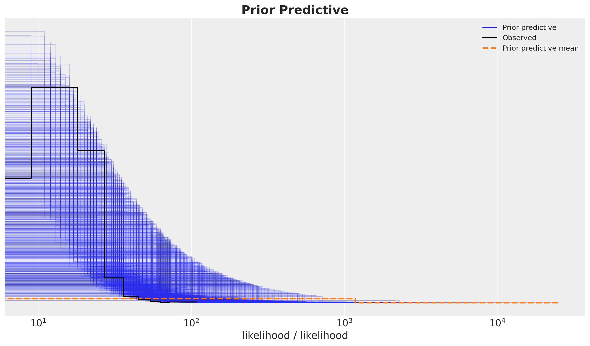
Overall the prior predictive looks reasonable.
Model Fitting
The model takes around \(10\) minutes to fit (Mac Book Pro, Intel Core i7).
with model:
    idata = pm.sample(
        tune=1_000,
        target_accept=0.90,
        draws=3_000,
        chains=4,
        random_seed=rng,
    )
    posterior_predictive = pm.sample_posterior_predictive(trace=idata, random_seed=rng)
Diagnostics
We look into the model diagnostics. First we check divergences:
idata["sample_stats"]["diverging"].sum().item()0No divergences! Let’s look into additional diagnostics:
var_names = [
    "power_minus",
    "power_plus",
    "sigma_is_release",
    "sigma_ell_is_release_minus",
    "sigma_ell_is_release_plus",
    "beta_is_release",
    "ell_is_release_minus",
    "ell_is_release_plus",
    "inv_alpha_lam",
    "inv_alpha",
    "alpha",
]

az.summary(data=idata, var_names=var_names, round_to=3)| mean | sd | hdi_3% | hdi_97% | mcse_mean | mcse_sd | ess_bulk | ess_tail | r_hat | |
|---|---|---|---|---|---|---|---|---|---|
| power_minus | 0.298 | 0.028 | 0.246 | 0.352 | 0.001 | 0.000 | 2391.351 | 4144.913 | 1.002 |
| power_plus | 0.252 | 0.020 | 0.215 | 0.288 | 0.002 | 0.001 | 86.111 | 1099.446 | 1.042 |
| sigma_is_release | 102.876 | 42.193 | 46.924 | 180.339 | 0.490 | 0.368 | 10416.997 | 6657.539 | 1.001 |
| sigma_ell_is_release_minus | 0.676 | 0.304 | 0.267 | 1.206 | 0.004 | 0.003 | 8418.883 | 6663.825 | 1.000 |
| sigma_ell_is_release_plus | 1.975 | 0.920 | 0.740 | 3.520 | 0.011 | 0.009 | 9682.738 | 7021.077 | 1.001 |
| beta_is_release[iphone_11] | 87.811 | 7.197 | 74.774 | 101.641 | 0.109 | 0.077 | 4319.084 | 6775.800 | 1.002 |
| beta_is_release[iphone_12] | 104.559 | 8.481 | 89.382 | 120.857 | 0.109 | 0.077 | 6011.804 | 7460.644 | 1.000 |
| beta_is_release[iphone_13] | 71.477 | 6.613 | 58.896 | 83.784 | 0.097 | 0.068 | 4645.736 | 6530.297 | 1.003 |
| beta_is_release[iphone_14] | 77.189 | 7.859 | 62.536 | 91.975 | 0.110 | 0.078 | 5044.312 | 7110.363 | 1.000 |
| ell_is_release_minus[iphone_11] | 0.306 | 0.092 | 0.090 | 0.443 | 0.003 | 0.002 | 887.354 | 876.292 | 1.005 |
| ell_is_release_minus[iphone_12] | 0.637 | 0.056 | 0.536 | 0.743 | 0.001 | 0.001 | 2138.258 | 3615.357 | 1.002 |
| ell_is_release_minus[iphone_13] | 0.508 | 0.054 | 0.405 | 0.610 | 0.002 | 0.001 | 1283.886 | 2246.039 | 1.010 |
| ell_is_release_minus[iphone_14] | 0.596 | 0.061 | 0.483 | 0.711 | 0.002 | 0.001 | 1061.666 | 2279.684 | 1.015 |
| ell_is_release_plus[iphone_11] | 1.621 | 0.165 | 1.323 | 1.932 | 0.004 | 0.003 | 1851.762 | 3902.532 | 1.005 |
| ell_is_release_plus[iphone_12] | 1.240 | 0.108 | 1.047 | 1.450 | 0.002 | 0.002 | 2247.391 | 4202.864 | 1.003 |
| ell_is_release_plus[iphone_13] | 1.653 | 0.164 | 1.358 | 1.965 | 0.003 | 0.002 | 2443.428 | 4825.193 | 1.003 |
| ell_is_release_plus[iphone_14] | 1.434 | 0.151 | 1.148 | 1.703 | 0.003 | 0.002 | 2339.363 | 4509.314 | 1.002 |
| inv_alpha_lam | 1063.267 | 343.859 | 455.498 | 1731.624 | 2.941 | 2.080 | 12516.787 | 5576.722 | 1.001 |
| inv_alpha[iphone_11] | 0.000 | 0.000 | 0.000 | 0.000 | 0.000 | 0.000 | 11882.618 | 6562.296 | 1.000 |
| inv_alpha[iphone_12] | 0.000 | 0.000 | 0.000 | 0.000 | 0.000 | 0.000 | 9734.909 | 5760.883 | 1.000 |
| inv_alpha[iphone_13] | 0.000 | 0.000 | 0.000 | 0.000 | 0.000 | 0.000 | 11053.589 | 5939.772 | 1.000 |
| inv_alpha[iphone_14] | 0.000 | 0.000 | 0.000 | 0.000 | 0.000 | 0.000 | 11624.208 | 6221.281 | 1.000 |
| alpha[iphone_11] | 145142.927 | 323221.101 | 14576.774 | 364749.684 | 4811.220 | 3442.385 | 11882.618 | 6562.296 | 1.000 |
| alpha[iphone_12] | 74385.878 | 189051.386 | 5906.571 | 193317.310 | 2613.356 | 1848.025 | 9734.909 | 5760.883 | 1.000 |
| alpha[iphone_13] | 44040.603 | 74711.095 | 4282.518 | 116911.536 | 995.960 | 704.287 | 11053.589 | 5939.772 | 1.000 |
| alpha[iphone_14] | 15155.624 | 24059.611 | 1308.656 | 40757.582 | 369.597 | 269.143 | 11624.208 | 6221.281 | 1.000 |
Overall, it looks fine.
axes = az.plot_trace(
    data=idata,
    var_names=var_names,
    compact=True,
    backend_kwargs={"figsize": (12, 15), "layout": "constrained"},
)
plt.gcf().suptitle("Model Trace", fontsize=18, fontweight="bold")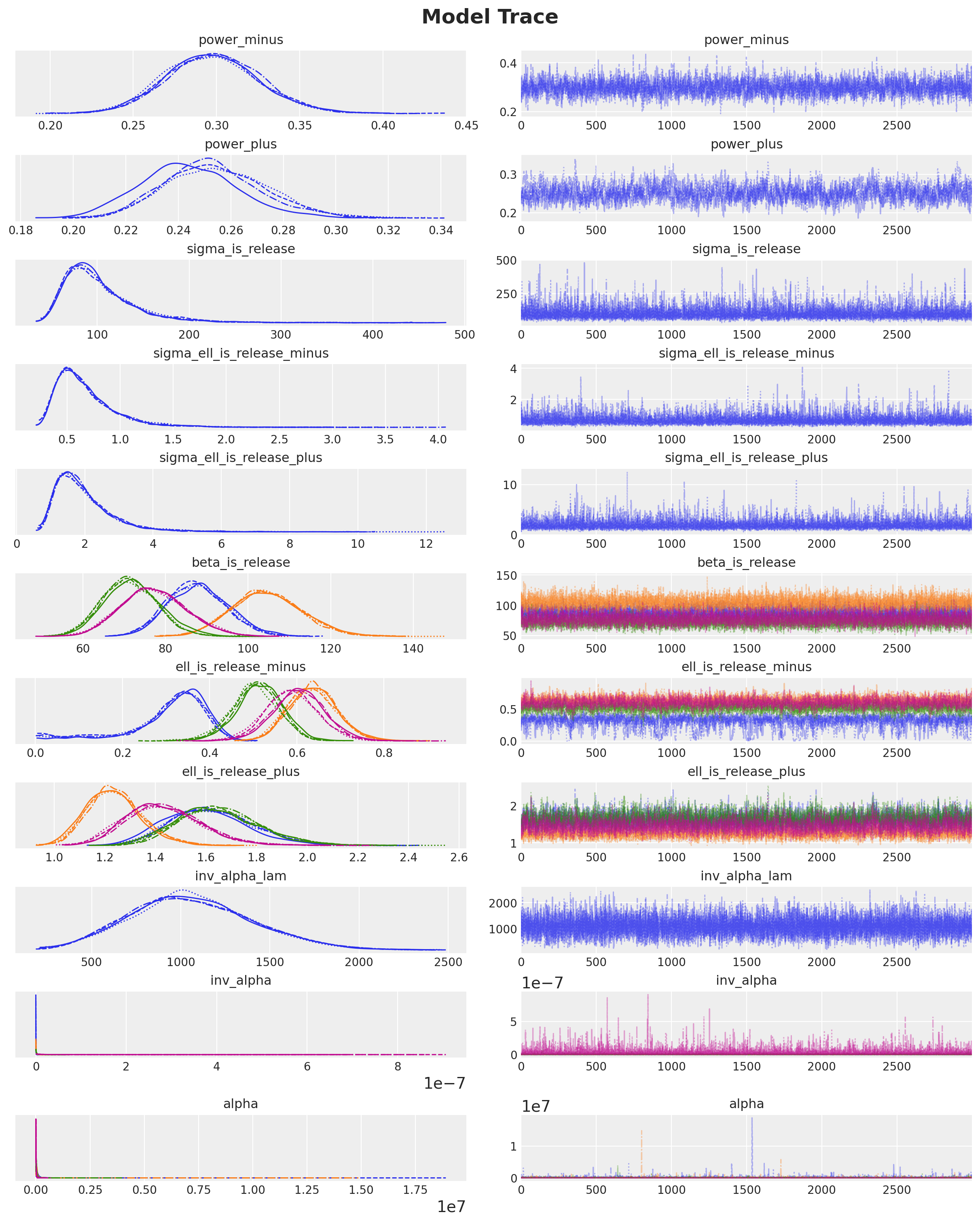
Posterior Predictive
We now look into the posterior predictive distribution:
az.plot_ppc(
    data=posterior_predictive,
    num_pp_samples=1_000,
    observed_rug=True,
    random_seed=seed,
)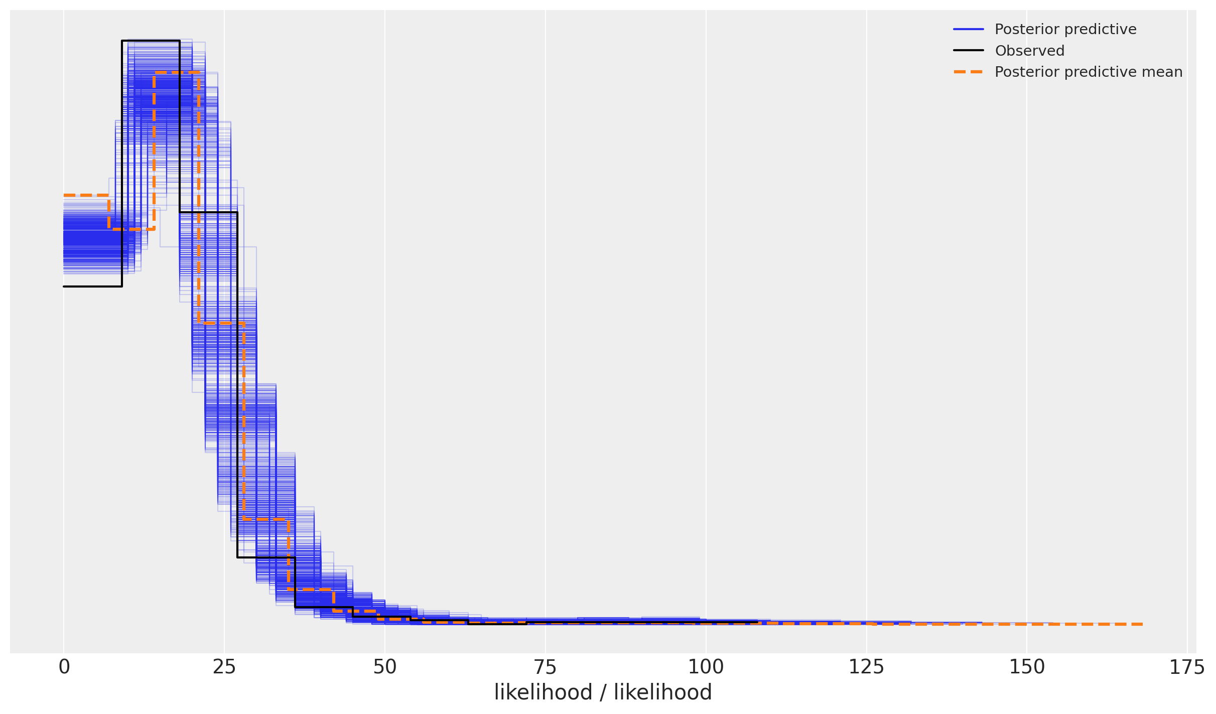
It looks the model has captured most of the variance from the data.
We can now look for each model separately:
fig, axes = plt.subplots(
    nrows=train_iphone_model.size,
    ncols=1,
    sharex=True,
    sharey=True,
    figsize=(12, 15),
    layout="constrained",
)

for i, iphone_model in enumerate(train_iphone_model):
    ax = axes[i]

    condition = train_df["model"] == iphone_model
    temp_df = train_df[condition]
    temp_likelihood = posterior_predictive["posterior_predictive"]["likelihood"][
        :, :, condition.to_numpy()
    ]

    sns.lineplot(
        data=temp_df,
        x="model_age",
        y="search",
        color="black",
        label="Observed",
        ax=ax,
    )
    sns.lineplot(
        x=temp_df["model_age"],
        y=temp_likelihood.mean(dim=("chain", "draw")),
        color=f"C{i}",
        label="Posterior Predictive Mean",
        ax=ax,
    )
    az.plot_hdi(
        x=temp_df["model_age"],
        y=temp_likelihood,
        hdi_prob=0.94,
        color=f"C{i}",
        smooth=False,
        fill_kwargs={"alpha": 0.3, "label": r"$94\%$ HDI"},
        ax=ax,
    )
    az.plot_hdi(
        x=temp_df["model_age"],
        y=temp_likelihood,
        hdi_prob=0.50,
        color=f"C{i}",
        smooth=False,
        fill_kwargs={"alpha": 0.6, "label": r"$50\%$ HDI"},
        ax=ax,
    )
    ax.legend(loc="upper right")
    ax.set(title=iphone_model, xlabel="Model Age (weeks)", ylabel="Search")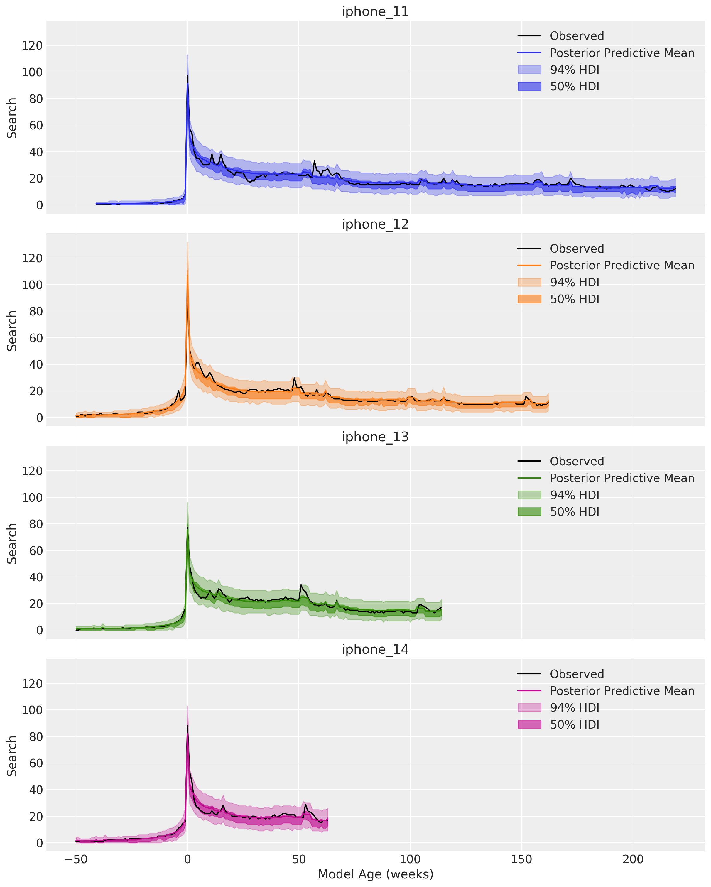
We indeed see we the model has captures the release peak, the decay and the yearly seasonality 🙌!
Life Cycle Components
We now split the posterior predictive mean into the release peak and decay components:
fig, ax = plt.subplots(figsize=(15, 7))

sns.lineplot(
    data=train_df,
    x="week",
    y="search",
    hue="model",
    ax=ax,
)

for i, iphone_model in enumerate(
    release_dates_df.query(f"model != '{test_model}'")["model"]
):
    condition = (train_df["model"] == iphone_model).to_numpy()

    release_week = release_dates_df.query(f"model == '{iphone_model}'")[
        "release_week"
    ].item()

    ax.axvline(
        release_week,
        color=f"C{i}",
        linestyle="--",
        label=f"release week {iphone_model}",
    )

    sns.lineplot(
        x=train_df["week"][condition],
        y=idata["posterior"]["is_release_bump"].mean(dim=("chain", "draw"))[condition],
        color=f"C{i}",
        alpha=0.5,
        label="Release Bump: (mean)",
        ax=ax,
    )

    sns.lineplot(
        x=train_df["week"][condition],
        y=np.exp(
            idata["posterior"]["bart_mu_log"].mean(dim=("chain", "draw"))[condition]
        ),
        color=f"C{i}",
        alpha=0.5,
        linestyle="-.",
        label="Decay component: (mean)",
        ax=ax,
    )

ax.legend(loc="upper center", bbox_to_anchor=(0.5, -0.12), ncol=3)
ax.set_title(
    label="Google Trends for iPhone Models (Worldwide)", fontsize=18, fontweight="bold"
)
Most of the variance is explained by the release Gaussian bump components. The decay component acs as a small collection over the initial peak decay.
We can decompose further de decay component by looking into the partial dependence plots:
axes = pmb.plot_pdp(
    bartrv=bart_mu_log,
    X=x_train,
    Y=train_search,
    func=np.exp,
    xs_interval="insample",
    samples=1_000,
    grid="long",
    color="C0",
    color_mean="C0",
    var_discrete=[2, 3, 4],
    figsize=(10, 12),
    random_seed=seed,
)
plt.gcf().suptitle(
    "Partial Dependency Plots (PDP)",
    fontsize=18,
    fontweight="bold",
    y=1.05,
)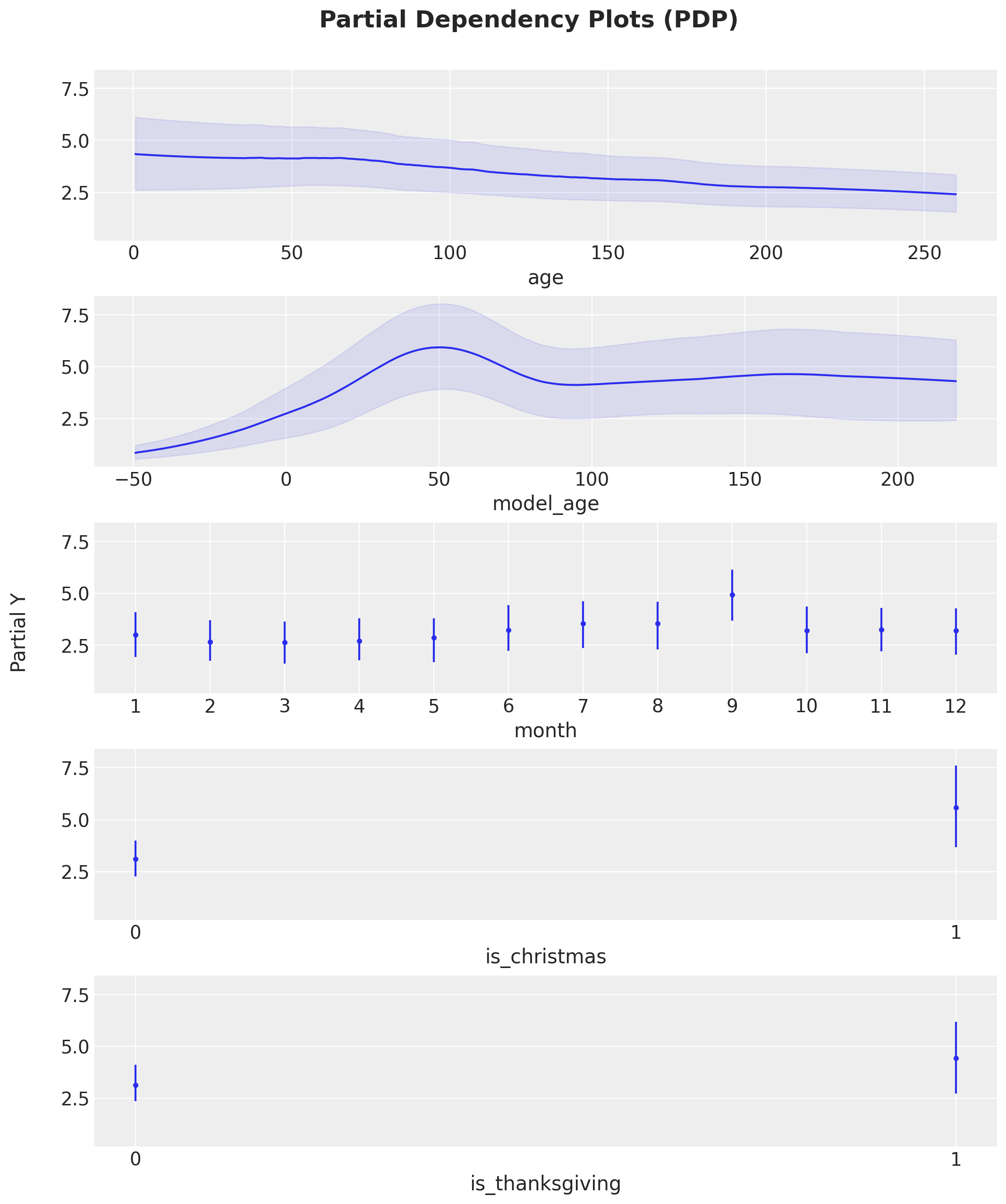
Here are some remarks from these partial dependence plots:
- Overall, the contribution of the decay component is small 9expected from the plot above).
- The age’s contribution decays monotonically.
- The variable model_age presents a bump around week \(50\), which seems to be be related to the release of the next iPhone model. We could add this feature to the model to capture this behavior.
- We see a mild seasonality contribution from the month variable, attaining a maximum around September when the new iPhone models are usually released.
- We also a mild contribution from the holidays variable. A better encoding would be a multiplicative interaction with the model age.
Out-of-Sample Predictions
We now generate out of sample prediction for the unseen iPhone model:
test_obs = test_df.index.to_numpy()
test_iphone_model_idx, test_iphone_model = test_df["model"].factorize(sort=True)
test_month_idx, test_month = test_df["month"].factorize(sort=True)
test_age = test_df["age"].to_numpy()
test_model_age = test_df["model_age"].to_numpy()
test_is_release = test_df["is_release"].to_numpy()
x_test = test_df[features]
test_search = test_df["search"].to_numpy()
with model:
pm.set_data(
new_data={
"iphone_model_idx_data": test_iphone_model_idx,
"model_age_data": test_model_age,
"x_data": x_test,
"search_data": np.ones_like(test_search), # Dummy data to make coords work!
# We are not using this at prediction time!
},
coords={"iphone_model": test_iphone_model, "obs": test_obs},
)
idata.extend(
pm.sample_posterior_predictive(
trace=idata,
var_names=["is_release_bump", "bart_mu_log", "likelihood"],
idata_kwargs={
"coords": {"iphone_model": test_iphone_model, "obs": test_obs}
},
random_seed=rng,
)
)Finally, we plot the posterior predictive distribution for the unseen iPhone model:
fig, ax = plt.subplots()

test_likelihood = idata["posterior_predictive"]["likelihood"]

i = 4

sns.lineplot(
    data=test_df,
    x="model_age",
    y="search",
    color="black",
    label="Observed",
    ax=ax,
)
sns.lineplot(
    x=test_df["model_age"],
    y=test_likelihood.mean(dim=("chain", "draw")),
    color=f"C{i}",
    label="Posterior Predictive Mean",
    ax=ax,
)
az.plot_hdi(
    x=test_df["model_age"],
    y=test_likelihood,
    hdi_prob=0.94,
    color=f"C{i}",
    smooth=False,
    fill_kwargs={"alpha": 0.3, "label": r"$94\%$ HDI"},
    ax=ax,
)
az.plot_hdi(
    x=test_df["model_age"],
    y=test_likelihood,
    hdi_prob=0.50,
    color=f"C{i}",
    smooth=False,
    fill_kwargs={"alpha": 0.6, "label": r"$50\%$ HDI"},
    ax=ax,
)
sns.lineplot(
    x=test_df["model_age"],
    y=idata["posterior_predictive"]["is_release_bump"].mean(dim=("chain", "draw")),
    color="C7",
    linewidth=2,
    alpha=0.7,
    label="Release Bump: Posterior Predictive Mean",
    ax=ax,
)
sns.lineplot(
    x=test_df["model_age"],
    y=np.exp(idata["posterior_predictive"]["bart_mu_log"].mean(dim=("chain", "draw"))),
    color="C7",
    linewidth=2,
    linestyle="-.",
    alpha=0.7,
    label="Decay component: Posterior Predictive Mean",
    ax=ax,
)
ax.legend(loc="upper left")
ax.set(title=test_model, xlabel="Model Age (weeks)", ylabel="Search")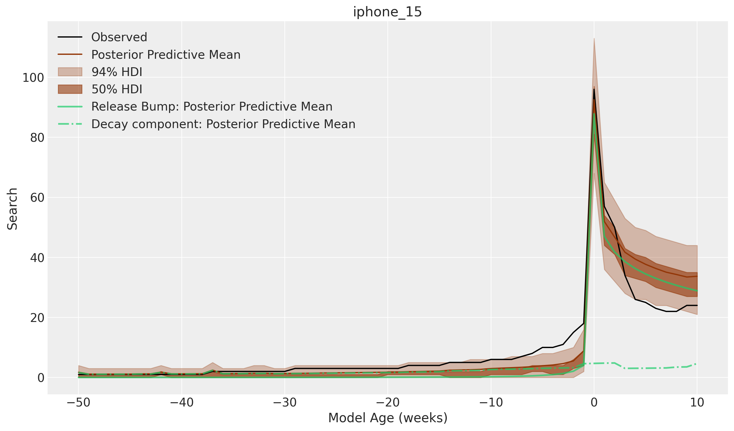
We see the model has captured the release peak and the decay within the \(94\%\) HDI. In particular, the predicted peak maximum is very close to the observed one.
Final Remarks
This example shows how to build a custom model for a family of products with similar life cycle structures. The model is flexible enough to capture the release peak and the long term decay. The model can be easily extended to other products and life cycle structures. Here we just illustrated some of the possibilities.