Prepare Notebook

import numpy as np
import pandas as pd
import matplotlib.pyplot as plt
import seaborn as sns
sns.set_style(
    style="darkgrid", 
    rc={"axes.facecolor": "0.9", "grid.color": "0.8"}
)
sns.set_palette(palette="deep")
sns_c = sns.color_palette(palette="deep")

plt.rcParams["figure.facecolor"] = "white"
plt.rcParams["figure.figsize"] = [10, 6]
plt.rcParams["figure.dpi"] = 100

%reload_ext autoreload
%autoreload 2

%config InlineBackend.figure_format = "svg"

Generate Sample Data

We generate a sample time series with a known trend, seasonal component, an external regressor and an auto-regressive term (see here for more details).

np.random.seed(1)

min_date = pd.to_datetime("2015-01-01")
max_date = pd.to_datetime("2022-01-01")

data_df = pd.DataFrame(
    data={"date": pd.date_range(start=min_date, end=max_date, freq="M")}
)

n = data_df.shape[0]

def generate_data(n, sigma_eta, sigma_epsilon):
   
    y = np.zeros(n)
    mu = np.zeros(n)
    epsilon = np.zeros(n)
    eta = np.zeros(n)

    for t in range(1, n):
        
        eta[t] = np.random.normal(loc=0.0, scale=sigma_eta)
        mu[t] = mu[t - 1] + eta[t]

        epsilon[t] = np.random.normal(loc=0.0, scale=sigma_epsilon)
        y[t] = mu[t] + epsilon[t]

    return y, mu

sigma_eta = 0.1
sigma_epsilon = 0.1

y, mu = generate_data(n=n, sigma_eta=sigma_eta, sigma_epsilon=sigma_epsilon)

data_df["y"] = y

# Add external regressor.
x = np.random.uniform(low=0.0, high=1.0, size=n)
data_df["x"] = np.where( x > 0.80, x, 0)
# Add seasonal component.
data_df["cs"] = np.sin(2 * np.pi * data_df["date"].dt.dayofyear / 356.5) 
data_df["cc"] = np.cos(3 * np.pi * data_df["date"].dt.dayofyear / 356.5) 
data_df["s"] = data_df["cs"] + data_df["cc"]
# Construct target variable.
data_df["z"] = data_df["y"] + data_df["x"] + data_df["s"]
# Add autoregressive term.
data_df["z"] = data_df["z"] + 0.5 * data_df["z"].shift(1).fillna(0)

Let us plot the time series and its components:

fig, ax = plt.subplots()
sns.lineplot(x="date", y="z", data=data_df, marker="o", markersize=5, color="black", label="z", ax=ax)
sns.lineplot(x="date", y="y", data=data_df, marker="o", markersize=5, color=sns_c[0], alpha=0.6, label="y (local level)", ax=ax)
sns.lineplot(x="date", y="s", data=data_df, marker="o", markersize=5, color=sns_c[1], alpha=0.6, label="seasonal", ax=ax)
sns.lineplot(x="date", y="x", data=data_df, marker="o", markersize=5, color=sns_c[2], alpha=0.6, label="x", ax=ax)
ax.legend(loc="center left", bbox_to_anchor=(1, 0.5))
ax.set(title="Simulated data components");

svg

Train-Test Split

Next we split the data into a training and test set.

# Set date as index.
data_df.set_index("date", inplace=True)
data_df.index = pd.DatetimeIndex(
    data=data_df.index.values,
    freq=data_df.index.inferred_freq
)

Let us see the split:

train_test_ratio = 0.80
n_train = int(n * train_test_ratio)
n_test = n - n_train

data_train_df = data_df[: n_train]
data_test_df = data_df[- n_test :]

y_train = data_train_df["z"]
x_train = data_train_df[["x"]]

y_test = data_test_df["z"]
x_test = data_test_df[["x"]]

fig, ax = plt.subplots()
sns.lineplot(x=y_train.index, y=y_train, marker="o", markersize=5, color=sns_c[0], label="y_train", ax=ax)
sns.lineplot(x=y_test.index, y=y_test, marker="o", markersize=5, color=sns_c[1], label="y_test", ax=ax)
ax.axvline(x=x_train.tail(1).index[0], color=sns_c[6], linestyle="--", label="train-test-split")
ax.legend(loc="center left", bbox_to_anchor=(1, 0.5))
ax.set(title="Train-Test Split");

svg

Fit Model

We not fit a UnobservedComponents model (also known as structural time series models). Recall that this is a model of the form:

\[ y_z = \mu_t + \gamma_t + c_t + \varepsilon_t \]

where \(\mu_t\) is the trend component, \(\gamma_t\) is the seasonal component, \(c_t\) is the cycle component and \(\varepsilon_t\) is the irregular component. Please see the great documentation for more details. For this specific case we will use \(4\) Fourier terms to model the yearly seasonality (similar to prophet). In addition, we are going to set the parameter mle_regression to True to add the external regressor into the state vector.

from statsmodels.tsa.statespace.structural import UnobservedComponents

model_params =  {
    "endog": y_train,
    "exog": x_train,
    "level": "local level",
    "freq_seasonal": [
         {"period": 12, "harmonics": 4}
    ],
    "autoregressive": 1,
    "mle_regression": True,
 }
 
model = UnobservedComponents(**model_params)

Let us now fit the model.

result = model.fit(disp=0)

result.summary()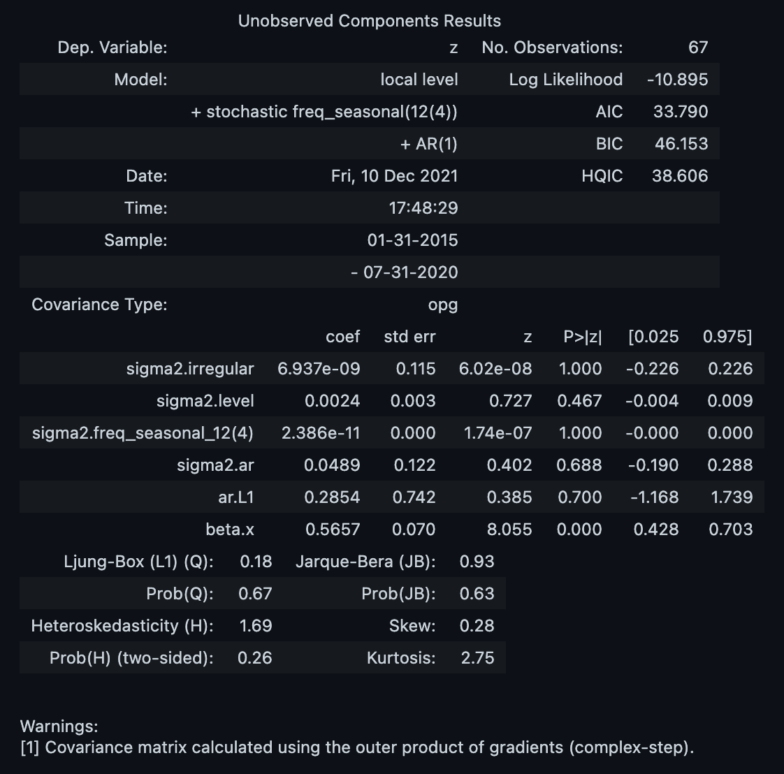

Now we can see some diagnostic plots:

result.plot_diagnostics(figsize=(12, 9));

svg

The error distribution looks ok! Now let us visualize the model (learned) components:

alpha = 0.05

fig = result.plot_components(figsize=(12, 9), alpha=alpha)

for ax in fig.get_axes():
    ax.legend(loc="center left", bbox_to_anchor=(1, 0.5))
    ax.set(title=None)

fig.suptitle("Model Components", y=0.92);

This decomposition agrees with our data generation process.

Remark: Let us get the number of observations needed for the approximate diffuse initialization (see here for more details).

n_obs_init = model.k_states - int(model._unused_state) - model.ar_order

Generate Predictions

Now we can use the fitted model to generate in and out sample predictions and confidence intervals.

train_predictions_summary = result \
    .get_prediction() \
    .summary_frame(alpha=alpha)

test_predictions_summary = result \
    .get_forecast(steps=n_test, exog=x_test) \
    .summary_frame(alpha=alpha)

Moreover, we can simulate from the state space model.

repetitions = 100

simulations_train_df = result.simulate(
    anchor="start",
    nsimulations=n_train,
    repetitions=repetitions,
    exog=x_train
)

simulations_test_df = result.simulate(
    anchor="end",
    nsimulations=n_test,
    repetitions=repetitions,
    exog=x_test
)

# Verify expected shape of the simulations dataframes.
assert simulations_train_df.shape == (n_train, repetitions)
assert simulations_test_df.shape == (n_test, repetitions)

Let us see the results:

fig, ax = plt.subplots()

# Input data
sns.lineplot(
    x=y_train.index,
    y=y_train,
    marker="o",
    markersize=5,
    color="C0",
    label="y_train",
    ax=ax
)
sns.lineplot(
    x=y_test.index,
    y=y_test,
    marker="o",
    markersize=5,
    color="C1",
    label="y_test",
    ax=ax
)
ax.axvline(
    x=x_train.tail(1).index[0],
    color="C6",
    linestyle="--",
    label="train-test-split"
)

# Simulations
for col in simulations_test_df.columns:
    sns.lineplot(
        x=simulations_test_df.index,
        y=simulations_test_df[col],
        color="C3",
        alpha=0.05, 
        ax=ax
    )

# Prediction intervals
ax.fill_between(
    x=train_predictions_summary.index[n_obs_init: ],
    y1=train_predictions_summary["mean_ci_lower"][n_obs_init: ],
    y2=train_predictions_summary["mean_ci_upper"][n_obs_init: ],
    color="C2",
    label="confidence interval (train)",
    alpha=0.3
)
ax.fill_between(
    x=test_predictions_summary.index[n_obs_init: ],
    y1=test_predictions_summary["mean_ci_lower"][n_obs_init: ],
    y2=test_predictions_summary["mean_ci_upper"][n_obs_init: ],
    color="C3",
    label="confidence interval (test)",
    alpha=0.3
)

# Predictions
sns.lineplot(
    x=train_predictions_summary.index,
    y=train_predictions_summary["mean"],
    marker="o",
    markersize=5,
    color="C2",
    label="y_train_pred",
    ax=ax
)
sns.lineplot(
    x=test_predictions_summary.index,
    y=test_predictions_summary["mean"],
    marker="o",
    markersize=5,
    color="C3",
    label="y_test_pred",
    ax=ax
)

# diffuse initialization
ax.axvline(
    x=y_train.index[n_obs_init],
    color="C5",
    linestyle="--",
    label="diffuse initialization"
)

ax.legend(loc="center left", bbox_to_anchor=(1, 0.5))
ax.set(title="Unobserved Components Model Predictions");

Here are some remarks:

• The in and out sample predictions look good and there is no sign of significant over-fit.
• Nevertheless, it seems that the models is underestimating the trend component a bit.
• Note that all the simulations lie withing the confidence intervals.

---

Write Model Wrapper

As mentioned in the introduction, we follow the indications of the post Fast Bayesian estimation of SARIMAX models to wrap the model as a PyMC model. Here is the main idea. The UnobservedComponents implementation from statsmodels already computes the derivative of the log-likelihood function with respect to the state vector. This is the main ingredient for the Hamiltonian Monte Carlo (HMC) algorithm. Hence, we just need to extract the likelihood and its derivate as a Theano / Aesara operator, which is what PyMC uses to construct the computational graph. To see the details about what is required to create a custom Python operator please see the extensive documentation Creating a new Op: Python implementation. The following is the structure of a Theano graph:

From the documentation:

Theano represents symbolic mathematical computations as graphs. Those graphs are bi-partite graphs (graphs with 2 types of nodes), they are composed of interconnected Apply and Variable nodes. Variable nodes represent data in the graph, either inputs, outputs or intermediary values. As such, Inputs and Outputs of a graph are lists of Theano Variable nodes. Apply nodes perform computation on these variables to produce new variables. Each Apply node has a link to an instance of Op which describes the computation to perform.

For our particular, we need to construct a Theano operator to compute the model’s likelihood and its derivative given a set of parameters. Concretely, we need to implement something of the form:

from theano.graph.op import Op

class Loglike(tt.Op):

    def __init__(self, model):
        ...

    def perform(self, node, inputs, outputs):
        """Compute log-likelihood."""
        ...

    def grad(self, inputs, g):
        """Compute gradient of log-likelihood (Jacobian)."""
        ...

See the description and requirements of the perform and grad methods respectively.

Now, how do we extract the likelihood from the UnobservedComponents model? We can access it via the loglike method. Let us compute the likelihood on the fitted parameters:

model.loglike(result.params)

-10.895206701947446

Similarly, we can compute the gradient of the likelihood via the score method.

model.score(params = result.params)

array([-6.72506452e+00, -1.14243319e-01, -4.49922733e+03,  2.79173498e-02,
        1.59160648e-05, -1.51104128e-03])

Note that the output is a vector as expected.

We first define a Score operator to compute the log-likelihood gradient:

import theano.tensor as tt

class Score(tt.Op):
    itypes = [tt.dvector]  # expects a vector of parameter values when called
    otypes = [tt.dvector]  # outputs vector of log-likelihood values

    def __init__(self, model):
        self.model = model

    def perform(self, node, inputs, outputs):
        (theta,) = inputs
        outputs[0][0] = self.model.score(theta)

Next we need a class to compute the likelihood.

class Loglike(tt.Op):

    itypes = [tt.dvector]  # expects a vector of parameter values when called
    otypes = [tt.dscalar]  # outputs a single scalar value (the log likelihood)

    def __init__(self, model):
        self.model = model
        self.score = Score(self.model)

    def perform(self, node, inputs, outputs):
        (theta,) = inputs  # contains the vector of parameters
        llf = self.model.loglike(theta)
        outputs[0][0] = np.array(llf)  # output the log-likelihood

    def grad(self, inputs, gradients):
        # the method that calculates the gradients - it actually returns the
        # vector-Jacobian product - gradients[0] is a vector of parameter values
        (theta,) = inputs  # our parameters
        out = [gradients[0] * self.score(theta)]
        return out

Remark: From the documentation The grad method must return a list containing one Variable for each input. Each returned Variable represents the gradient with respect to that input computed based on the symbolic gradients with respect to each output.

We are now ready to write the wrapper:

loglike = Loglike(model)

Let us see this in action:

# parameters to theano tensor
tt_params =  tt.as_tensor_variable(x=result.params.to_numpy(), ndim=1)

# We evaluate the log-likelihood
type(loglike(tt_params))

theano.tensor.var.TensorVariable

# To get the value we evaluate the tensor
loglike(tt_params).eval()

array(-10.8952067)

Run PyMC Model

In order to write the PyMC model we need to define a target distribution. In this case we can use DensityDist which is a distribution with the passed log density function is created.

import arviz as az
import pymc3 as pm

# Set sampling params
ndraws = 4000  # number of draws from the distribution
nburn = 1000  # number of "burn-in points" (which will be discarded)

with pm.Model() as pm_model:
    # Priors
    sigma2_irregular = pm.InverseGamma("sigma2.irregular", alpha=2, beta=1)
    sigma2_level = pm.InverseGamma("sigma2.level", alpha=2, beta=1)
    sigma2_freq_seasonal = pm.InverseGamma("sigma2.freq_seasonal_12(4)", alpha=2, beta=1)
    sigma2_ar = pm.InverseGamma("sigma2.ar", alpha=2, beta=1)
    ar_L1 = pm.Uniform("ar.L1", lower=-0.99, upper=0.99)
    beta_x = pm.Normal("beta.x", mu=0, sigma=1)

    # convert variables to tensor vectors
    theta = tt.as_tensor_variable([
        sigma2_irregular,
        sigma2_level,
        sigma2_freq_seasonal,
        sigma2_ar,
        ar_L1,
        beta_x
    ])

    # use a DensityDist (use a lamdba function to "call" the Op)
    pm.DensityDist("likelihood", logp=loglike, observed=theta)

Let us see the model structure:

pm_model

\[ \begin{array}{rcl} \text{sigma2.irregular_log__} &\sim & \text{TransformedDistribution}\\\text{sigma2.level_log__} &\sim & \text{TransformedDistribution}\\\text{sigma2.freq_seasonal_12(4)_log__} &\sim & \text{TransformedDistribution}\\\text{sigma2.ar_log__} &\sim & \text{TransformedDistribution}\\\text{ar.L1_interval__} &\sim & \text{TransformedDistribution}\\\text{beta.x} &\sim & \text{Normal}\\\text{sigma2.irregular} &\sim & \text{InverseGamma}\\\text{sigma2.level} &\sim & \text{InverseGamma}\\\text{sigma2.freq_seasonal_12(4)} &\sim & \text{InverseGamma}\\\text{sigma2.ar} &\sim & \text{InverseGamma}\\\text{ar.L1} &\sim & \text{Uniform}\\\text{likelihood} &\sim & \text{DensityDist} \end{array} \]

Next, we fit the model:

with pm_model:

    trace = pm.sample(
        draws=ndraws,
        tune=nburn,
        chains=4,
        return_inferencedata=True,
        cores=-1,
        compute_convergence_checks=True,
    )

We can now plot the trace of the model and compare them against the point estimate of the maximu likelihood estimations from the statsmodels implementation:

az.plot_trace(
    data=trace,
    lines=[(k, {}, [v]) for k, v in dict(result.params).items()]
)
plt.tight_layout()

Note that all the sigma2.* variables have much larger values in the pymc model. This is also the case in some of the models of the original statsmodels post.

We can now compute some diagnostics metrics as usual (see this post on Introduction to Bayesian Modeling with PyMC3:

az.summary(trace)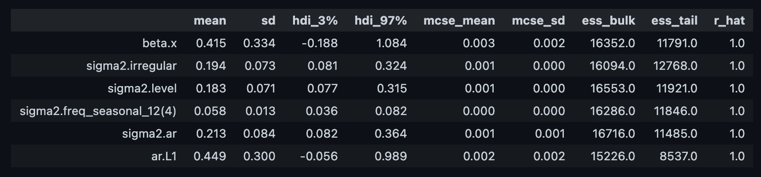

Let us compare with the original model parameters:

result.params

sigma2.irregular              6.936593e-09
sigma2.level                  2.357237e-03
sigma2.freq_seasonal_12(4)    2.385904e-11
sigma2.ar                     4.892693e-02
ar.L1                         2.854379e-01
beta.x                        5.656842e-01
dtype: float64

Generate Predictions

Now ge generate predictions by sampling from the posterior distribution. First, we take a subset of samples.

# number os samples
n_samples = 200

# sample with replacement from the posterior
posterior_samples = trace["posterior"] \
    .stack(sample=("chain", "draw")) \
    .to_pandas() \
    .sample(n=n_samples, replace=True)

# make sure the parameters are in the right order
posterior_samples = posterior_samples[result.params.index.to_numpy()]

For these samples we just update the parameters of the model using the (Kalman) smooth method.

pm_models = []

for i in range(n_samples):
    params = posterior_samples.iloc[i].to_numpy()
    result_bayes = model.smooth(params=params)
    pm_models.append(result_bayes)

# get in-sample fitted values
train_fitted_values_df = pd.concat(
    [m.fittedvalues[n_obs_init: ] for m in pm_models],
axis=1)

# get out-of-sample forecasted values
test_predicted_values_df = pd.concat(
    [m.forecast(steps=n_test, exog=x_test) for m in pm_models],
axis=1)
test_predicted_values_df.columns = [f"c_{i}" for i in range(n_samples)]

# simulate from the model
sim_test_df  = pd.concat(
    [
        m.simulate(
            anchor="end",
            nsimulations=n_test,
            repetitions=1,
            exog=x_test
        )
        for m in pm_models
    ],
axis=1)
sim_test_df.columns = [f"c_{i}" for i in range(n_samples)]

Finally, let us visualize the final results:

fig, ax = plt.subplots(figsize=(12, 7))

# Input data
sns.lineplot(
    x=y_train.index,
    y=y_train,
    marker="o",
    markersize=5,
    color=sns_c[0],
    label="y_train",
    ax=ax
)
sns.lineplot(
    x=y_test.index,
    y=y_test,
    marker="o",
    markersize=5,
    color=sns_c[1],
    label="y_test",
    ax=ax
)
ax.axvline(
    x=x_train.tail(1).index[0],
    color=sns_c[6],
    linestyle="--",
    label="train-test-split"
)

# Predictions

for i, col in enumerate(train_fitted_values_df.columns):

    label = "fitted values" if i == 0 else None
    sns.lineplot(
        x=train_fitted_values_df.index,
        y=train_fitted_values_df[col],
        color="C2",
        alpha=0.03,
        label=label,
        ax=ax
    )

for i, col in enumerate(test_predicted_values_df.columns):
    label = "predicted values" if i == 0 else None
    sns.lineplot(
        x=test_predicted_values_df.index,
        y=test_predicted_values_df[col],
        color="C3",
        alpha=0.03,
        label=label,
        ax=ax
    )

for i, col in enumerate(sim_test_df.columns):
    label = "simulated value" if i == 0 else None
    sns.lineplot(
        x=sim_test_df.index,
        y=sim_test_df[col],
        color="C3",
        alpha=0.03,
        label=label,
        ax=ax
    )

# diffuse initialization
ax.axvline(
    x=y_train.index[n_obs_init],
    color="C5",
    linestyle="--",
    label="diffuse initialization"
)
ax.legend(loc="center left", bbox_to_anchor=(1, 0.5))
ax.set(title="Unobserved Components PyMC Model Predictions");

Note that the simulated out-of-sample predictions range is much wider than the frequentist results as we are also considering the uncertainty of the model fitted parameters from the posterior distribution.