From Pyro to NumPyro: Forecasting Hierarchical Models - Part II

Prepare Notebook

import arviz as az
import jax
import jax.numpy as jnp
import matplotlib.pyplot as plt
import numpyro
import numpyro.distributions as dist
from jax import random
from jaxtyping import Array, Float
from numpyro.contrib.control_flow import scan
from numpyro.infer import SVI, Predictive, Trace_ELBO
from numpyro.infer.autoguide import AutoNormal
from numpyro.infer.reparam import LocScaleReparam
from pyro.contrib.examples.bart import load_bart_od

az.style.use("arviz-darkgrid")
plt.rcParams["figure.figsize"] = [12, 7]
plt.rcParams["figure.dpi"] = 100
plt.rcParams["figure.facecolor"] = "white"

numpyro.set_host_device_count(n=4)

rng_key = random.PRNGKey(seed=42)

%load_ext autoreload
%autoreload 2
%load_ext jaxtyping
%jaxtyping.typechecker beartype.beartype
%config InlineBackend.figure_format = "retina"

The autoreload extension is already loaded. To reload it, use:
  %reload_ext autoreload
The jaxtyping extension is already loaded. To reload it, use:
  %reload_ext jaxtyping

Read Data

dataset = load_bart_od()
print(dataset.keys())
print(dataset["counts"].shape)
print(" ".join(dataset["stations"]))

dict_keys(['stations', 'start_date', 'counts'])
torch.Size([78888, 50, 50])
12TH 16TH 19TH 24TH ANTC ASHB BALB BAYF BERY CAST CIVC COLM COLS CONC DALY DBRK DELN DUBL EMBR FRMT FTVL GLEN HAYW LAFY LAKE MCAR MLBR MLPT MONT NBRK NCON OAKL ORIN PCTR PHIL PITT PLZA POWL RICH ROCK SANL SBRN SFIA SHAY SSAN UCTY WARM WCRK WDUB WOAK

In this second example, we model all the rides from all stations to all other stations.

data = dataset["counts"].permute(1, 2, 0).log1p()
T = data.shape[-2]
print(data.shape)

torch.Size([50, 50, 78888])

Train - Test Split

Similarly as in the first example, for training purposes we will use data from 90 days before the test data.

T2 = data.size(-1)  # end
T1 = T2 - 24 * 7 * 2  # train/test split
T0 = T1 - 24 * 90  # beginning: train on 90 days of data

y = jnp.array(data[..., T0:T2])
y_train = jnp.array(data[..., T0:T1])
y_test = jnp.array(data[..., T1:T2])

print(f"y: {y.shape}")
print(f"y_train: {y_train.shape}")
print(f"y_test: {y_test.shape}")

y: (50, 50, 2496)
y_train: (50, 50, 2160)
y_test: (50, 50, 336)

n_stations = y_train.shape[-2]

time = jnp.array(range(T0, T2))
time_train = jnp.array(range(T0, T1))
t_max_train = time_train.size

time_test = jnp.array(range(T1, T2))
t_max_test = time_test.size

covariates = jnp.zeros_like(y)
covariates_train = jnp.zeros_like(y_train)
covariates_test = jnp.zeros_like(y_test)

assert time_train.size + time_test.size == time.size
assert y_train.shape == (n_stations, n_stations, t_max_train)
assert y_test.shape == (n_stations, n_stations, t_max_test)
assert covariates.shape == y.shape
assert covariates_train.shape == y_train.shape
assert covariates_test.shape == y_test.shape

Repeating Seasonal Features

We also need the JAX version of the periodic_repeat function.

def periodic_repeat_jax(tensor: Array, size: int, dim: int) -> Array:
    """
    Repeat a period-sized tensor up to given size using JAX.

    Parameters
    ----------
    tensor : Array
        A JAX array to be repeated.
    size : int
        Desired size of the result along dimension `dim`.
    dim : int
        The tensor dimension along which to repeat.

    Returns
    -------
    Array
        The repeated tensor.

    References
    ----------
    Thttps://docs.pyro.ai/en/stable/ops.html#pyro.ops.tensor_utils.periodic_repeat
    """
    assert isinstance(size, int) and size >= 0
    assert isinstance(dim, int)
    if dim >= 0:
        dim -= tensor.ndim

    period = tensor.shape[dim]
    repeats = [1] * tensor.ndim
    repeats[dim] = (size + period - 1) // period
    result = jnp.tile(tensor, repeats)

    slices = [slice(None)] * tensor.ndim
    slices[dim] = slice(None, size)

    return result[tuple(slices)]

Model Specification

In this model, the local level dynamic is driven by the destination station. On the other hand, the seasonal components and the noise scales come as a sum of the origin and destination stations. The model structure is very similar to the one presented in the first example.

def model(
    covariates: Float[Array, "n_series n_series t_max"],
    y: Float[Array, "n_series n_series t_max"] | None = None,
) -> None:
    # Get the time and feature dimensions
    n_series, n_series, t_max = covariates.shape

    # Define the plates to be able to use them below
    origin_plate = numpyro.plate("origin", n_series, dim=-3)
    destin_plate = numpyro.plate("destin", n_series, dim=-2)
    hour_of_week_plate = numpyro.plate("hour_of_week", 24 * 7, dim=-1)

    # Global scale for the drift
    drift_scale = numpyro.sample("drift_scale", dist.LogNormal(loc=-20, scale=5))

    # Sample the centered parameter for the LocScaleReparam
    destin_centered = numpyro.sample("destin_centered", dist.Uniform(low=0, high=1))

    with origin_plate, hour_of_week_plate:
        origin_seasonal = numpyro.sample("origin_seasonal", dist.Normal(loc=0, scale=5))

    with destin_plate:
        with (
            numpyro.plate("time", t_max),
            numpyro.handlers.reparam(
                config={"drift": LocScaleReparam(centered=destin_centered)}
            ),
        ):
            # Sample the drift parameters
            # We have one drift parameter per time series (station) and time point
            drift = numpyro.sample("drift", dist.Normal(loc=0, scale=drift_scale))

        with hour_of_week_plate:
            # Sample the seasonal parameters
            # We have one seasonal parameter per hour of the week and per station
            destin_seasonal = numpyro.sample(
                "destin_seasonal", dist.Normal(loc=0, scale=5)
            )

    # We model a static pairwise station->station affinity, which e.g.
    # can compensate for the fact that people tend not to travel from
    # a station to itself.
    with origin_plate, destin_plate:
        pairwise = numpyro.sample("pairwise", dist.Normal(0, 1))

    # We model the origin and destination scales separately
    # and then add them together to get the final scale.
    with origin_plate:
        origin_scale = numpyro.sample("origin_scale", dist.LogNormal(-5, 5))
    with destin_plate:
        destin_scale = numpyro.sample("destin_scale", dist.LogNormal(-5, 5))
        scale = origin_scale + destin_scale

    # Repeat the seasonal parameters to match the length of the time series
    seasonal = origin_seasonal + destin_seasonal
    seasonal_repeat = periodic_repeat_jax(seasonal, t_max, dim=-1)

    # Define the local level transition function
    def transition_fn(carry, t):
        "Local level transition function"
        previous_level = carry
        current_level = previous_level + drift[..., t]
        return current_level, current_level

    # Compute the latent levels using scan
    _, pred_levels = scan(
        transition_fn, init=jnp.zeros((n_series,)), xs=jnp.arange(t_max)
    )

    # We need to transpose the prediction levels to match the shape of the data
    pred_levels = pred_levels.transpose(1, 0)

    # Compute the mean of the model
    mu = pred_levels + seasonal_repeat + pairwise

    # Sample the observations
    with numpyro.handlers.condition(data={"obs": y}):
        numpyro.sample("obs", dist.Normal(loc=mu, scale=scale))

We can now visualize the model structure.

numpyro.render_model(
    model=model,
    model_kwargs={"covariates": covariates_train, "y": y_train},
    render_distributions=True,
    render_params=True,
)

Prior Predictive Checks

As usual (highly recommended!), we should perform prior predictive checks.

prior_predictive = Predictive(model=model, num_samples=500, return_sites=["obs"])

rng_key, rng_subkey = random.split(rng_key)

prior_samples = prior_predictive(rng_subkey, covariates_train)

idata_prior = az.from_dict(
    prior_predictive={k: v[None, ...] for k, v in prior_samples.items()},
    coords={
        "time_train": time_train,
        "origin": dataset["stations"],
        "destin": dataset["stations"],
    },
    dims={"obs": ["origin", "destin", "time_train"]},
)

Let’s plot the prior predictive distribution for the first \(8\) stations for the destination station ANTC.

station = "ANTC"
idx = dataset["stations"].index(station)

fig, axes = plt.subplots(
    nrows=8, ncols=1, figsize=(15, 18), sharex=True, sharey=True, layout="constrained"
)
for i, ax in enumerate(axes):
    for j, hdi_prob in enumerate([0.94, 0.5]):
        az.plot_hdi(
            time_train[time_train >= T1 - 3 * (24 * 7)],
            idata_prior["prior_predictive"]["obs"]
            .sel(destin=station)
            .isel(origin=i)[:, :, time_train >= T1 - 3 * (24 * 7)]
            .clip(min=0),
            hdi_prob=hdi_prob,
            color="C0",
            fill_kwargs={
                "alpha": 0.3 + 0.2 * j,
                "label": f"{hdi_prob*100:.0f}% HDI (train)",
            },
            smooth=False,
            ax=ax,
        )

    ax.plot(
        time_train[time_train >= T1 - 3 * (24 * 7)],
        data[i, idx, T1 - 3 * (24 * 7) : T1],
        "black",
        lw=1,
        label="Truth",
    )

    ax.legend(
        bbox_to_anchor=(1.05, 1), loc="upper left", borderaxespad=0.0, fontsize=12
    )

fig.suptitle("Prior predictive checks", fontsize=18, fontweight="bold");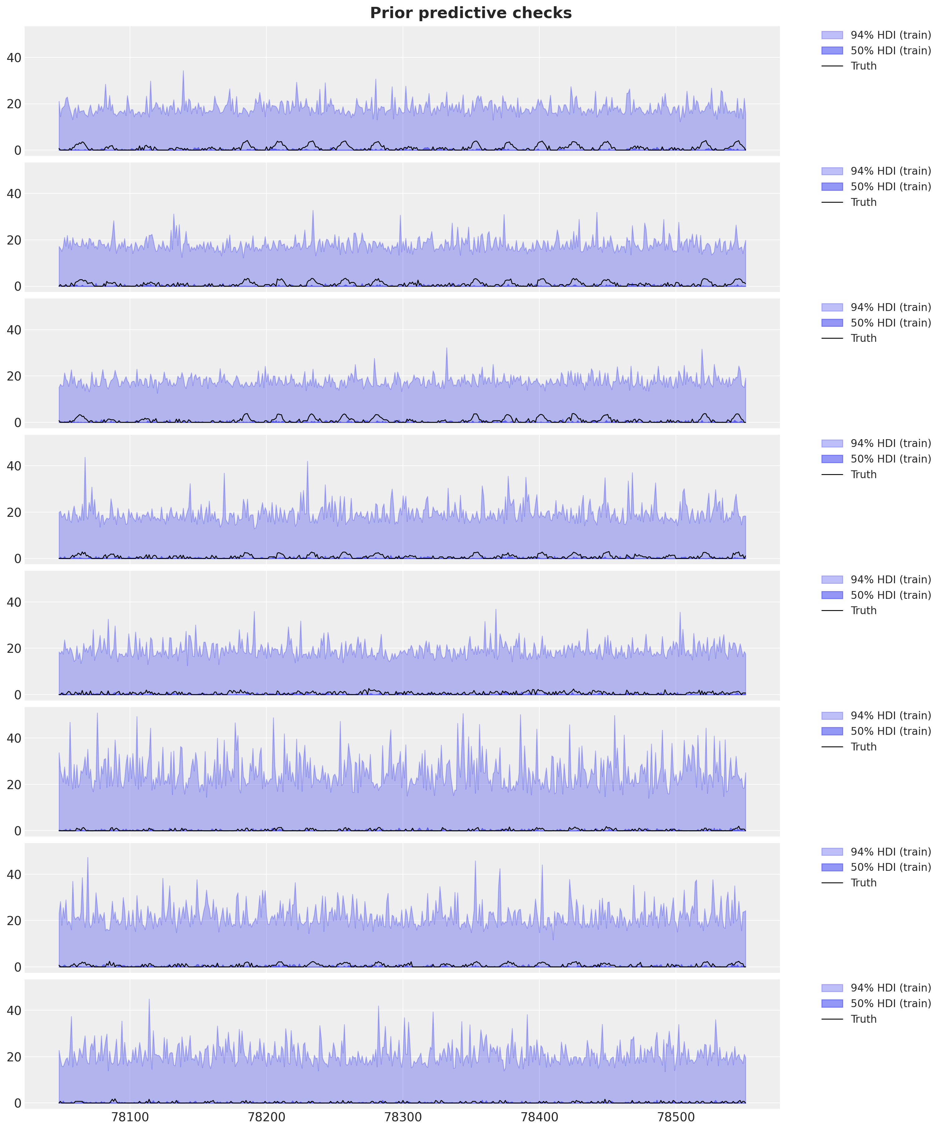

Overall, the prior ranges look very reasonable (even too wide).

Inference with SVI

We now fit the model to the data using stochastic variational inference. This time the model runs for longer as compared to the first one (\(45\) seconds to \(3.5\) minutes).

%%time

guide = AutoNormal(model)
optimizer = numpyro.optim.Adam(step_size=0.1)
svi = SVI(model, guide, optimizer, loss=Trace_ELBO())
num_steps = 10_000

rng_key, rng_subkey = random.split(key=rng_key)

svi_result = svi.run(
    rng_subkey,
    num_steps,
    covariates_train,
    y_train,
)

fig, ax = plt.subplots(figsize=(9, 6))
ax.plot(svi_result.losses)
ax.set_yscale("log")
ax.set_title("ELBO loss", fontsize=18, fontweight="bold");

100%|██████████| 10000/10000 [03:23<00:00, 49.10it/s, init loss: 1727067648.0000, avg. loss [9501-10000]: 3742141.6960]


CPU times: user 9min 45s, sys: 1min 46s, total: 11min 31s
Wall time: 3min 28s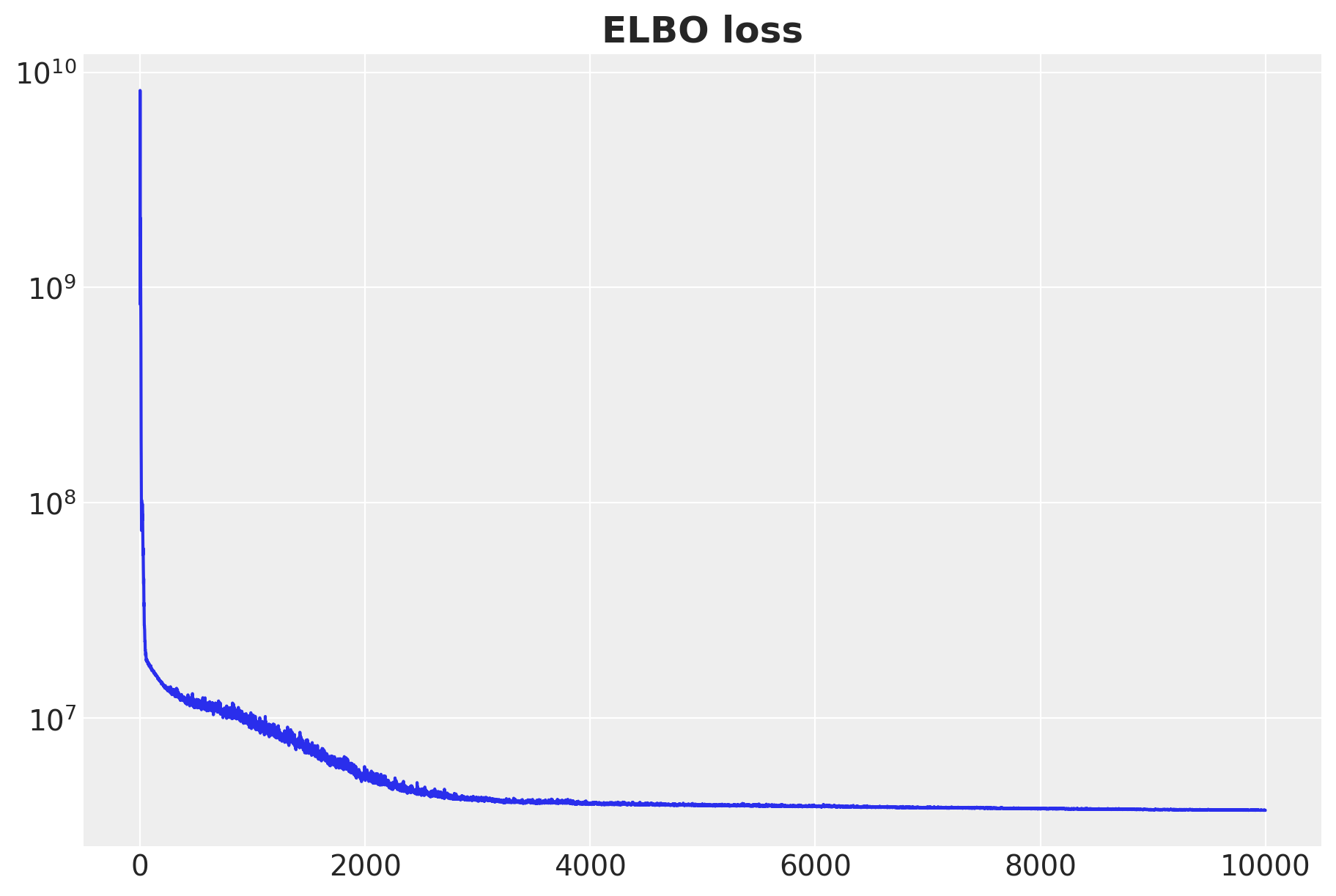

The resulting ELBO loss good!

Posterior Predictive Check

Next, we generate posterior predictive samples for the forecast for each of the stations pairs.

posterior = Predictive(
    model=model,
    guide=guide,
    params=svi_result.params,
    num_samples=200,
    return_sites=["obs"],
)

rng_key, rng_subkey = random.split(rng_key)

idata_train = az.from_dict(
    posterior_predictive={
        k: v[None, ...] for k, v in posterior(rng_subkey, covariates_train).items()
    },
    coords={
        "time_train": time_train,
        "origin": dataset["stations"],
        "destin": dataset["stations"],
    },
    dims={"obs": ["origin", "destin", "time_train"]},
)

idata_test = az.from_dict(
    posterior_predictive={
        k: v[None, ...] for k, v in posterior(rng_subkey, covariates).items()
    },
    coords={
        "time": time,
        "origin": dataset["stations"],
        "destin": dataset["stations"],
    },
    dims={"obs": ["origin", "destin", "time"]},
)

To evaluate the model performance,we compute the CRPS for the training and test data. For comparison purposes, we clip the data to ensure the predictions are non-negative.

@jax.jit
def crps(
    truth: Float[Array, "n_series n_series t_max"],
    pred: Float[Array, "n_samples n_series n_series t_max"],
    sample_weight: Float[Array, " t_max"] | None = None,
) -> Float[Array, ""]:
    if pred.shape[1:] != (1,) * (pred.ndim - truth.ndim - 1) + truth.shape:
        raise ValueError(
            f"""Expected pred to have one extra sample dim on left.
            Actual shapes: {pred.shape} versus {truth.shape}"""
        )

    absolute_error = jnp.mean(jnp.abs(pred - truth), axis=0)

    num_samples = pred.shape[0]
    if num_samples == 1:
        return jnp.average(absolute_error, weights=sample_weight)

    pred = jnp.sort(pred, axis=0)
    diff = pred[1:] - pred[:-1]
    weight = jnp.arange(1, num_samples) * jnp.arange(num_samples - 1, 0, -1)
    weight = weight.reshape(weight.shape + (1,) * (diff.ndim - 1))

    per_obs_crps = absolute_error - jnp.sum(diff * weight, axis=0) / num_samples**2
    return jnp.average(per_obs_crps, weights=sample_weight)


crps_train = crps(
    y_train,
    jnp.array(idata_train["posterior_predictive"]["obs"].sel(chain=0).clip(min=0)),
)

crps_test = crps(
    y_test,
    jnp.array(
        idata_test["posterior_predictive"]["obs"]
        .sel(chain=0)
        .sel(time=slice(T1, T2))
        .clip(min=0)
    ),
)

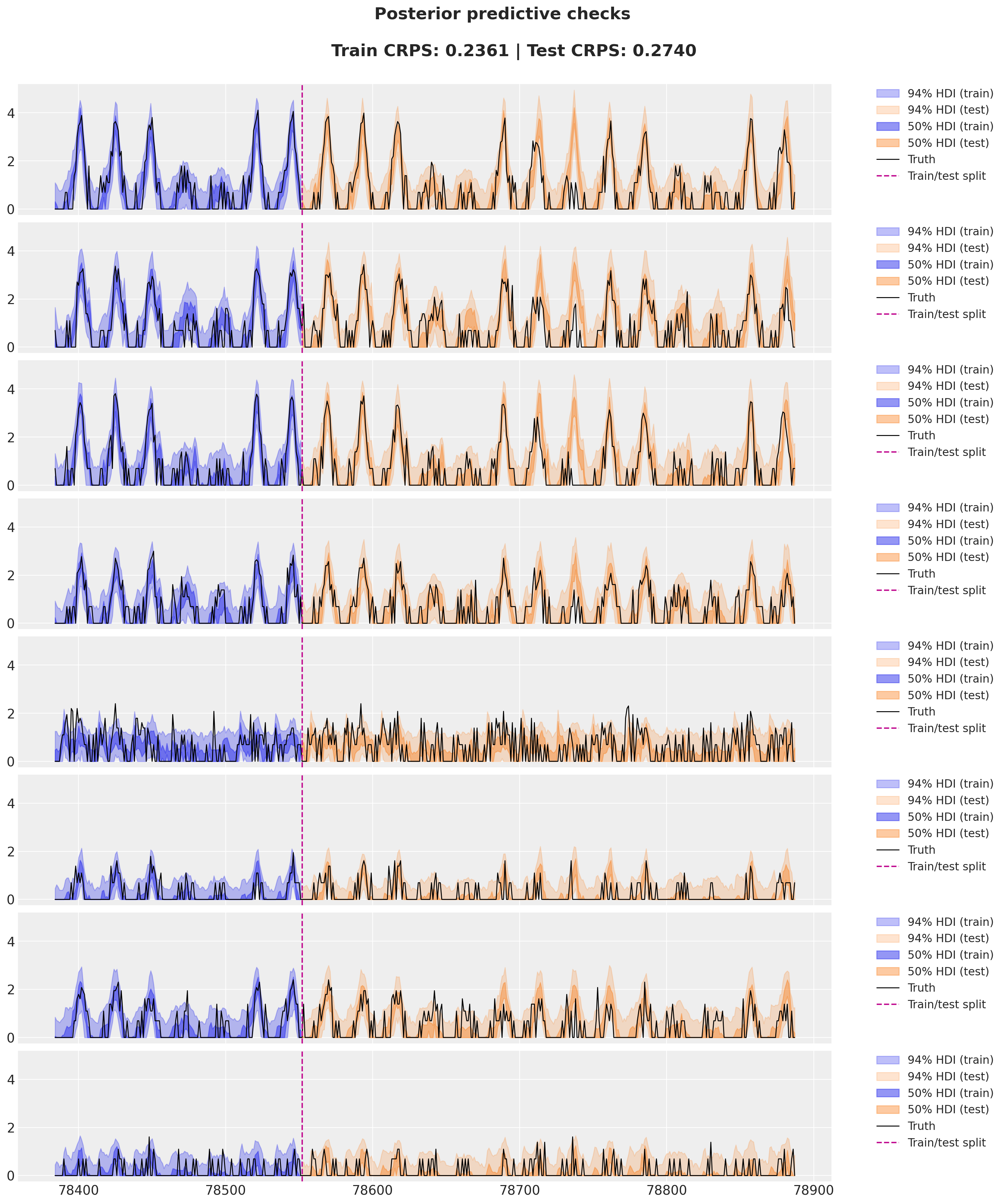
Finally, we reproduce the model fit and plot from the Pyro example.

station = "ANTC"
idx = dataset["stations"].index(station)

fig, axes = plt.subplots(
    nrows=8, ncols=1, figsize=(15, 18), sharex=True, sharey=True, layout="constrained"
)
for i, ax in enumerate(axes):
    for j, hdi_prob in enumerate([0.94, 0.5]):
        az.plot_hdi(
            time_train[time_train >= T1 - 24 * 7],
            idata_train["posterior_predictive"]["obs"]
            .sel(destin=station)
            .isel(origin=i)[:, :, time_train >= T1 - 24 * 7]
            .clip(min=0),
            hdi_prob=hdi_prob,
            color="C0",
            fill_kwargs={
                "alpha": 0.3 + 0.2 * j,
                "label": f"{hdi_prob*100:.0f}% HDI (train)",
            },
            smooth=False,
            ax=ax,
        )

        az.plot_hdi(
            time[time >= T1],
            idata_test["posterior_predictive"]["obs"]
            .sel(destin=station)
            .isel(origin=i)[:, :, time >= T1]
            .clip(min=0),
            hdi_prob=hdi_prob,
            color="C1",
            fill_kwargs={
                "alpha": 0.2 + 0.2 * j,
                "label": f"{hdi_prob*100:.0f}% HDI (test)",
            },
            smooth=False,
            ax=ax,
        )

    ax.plot(
        time[time >= T1 - 24 * 7],
        data[i, idx, T1 - 24 * 7 : T2],
        "black",
        lw=1,
        label="Truth",
    )

    ax.axvline(T1, color="C3", linestyle="--", label="Train/test split")

    ax.legend(
        bbox_to_anchor=(1.05, 1), loc="upper left", borderaxespad=0.0, fontsize=12
    )

fig.suptitle(
    f"""Posterior predictive checks

    Train CRPS: {crps_train:.4f} | Test CRPS: {crps_test:.4f}
    """,
    fontsize=18,
    fontweight="bold",
);