In this notebooks we port the Pyro forecasting example Forecasting I: univariate, heavy tailed to NumPyro. The forecasting module in Pyro is fantastic as it provides an easy interface to develop custom forecasting models. It has also many helpful utility functions to generate features and for model evaluation. The purpose of this translation is to dig deeper into the some forecasting components and to show that translating Pyro code to NumPyro is not that hard, even though there are come caveats.
The original Pyro example provides a great introduction to some univariate forecasting models. In particular, it provides various iterations from simple models to more complex models. We do not aim to repeat the already existing examples, but to focus on the forecasting components of the final model.
Prepare Notebook
from typing import Any

import arviz as az
import jax.numpy as jnp
import matplotlib.pyplot as plt
import numpyro
import numpyro.distributions as dist
from jax import random
from jaxtyping import Array, Float
from numpyro.contrib.control_flow import scan
from numpyro.infer import SVI, Predictive, Trace_ELBO
from numpyro.infer.autoguide import AutoNormal
from numpyro.infer.reparam import LocScaleReparam
from pyro.contrib.examples.bart import load_bart_od
from pyro.ops.tensor_utils import periodic_features

az.style.use("arviz-darkgrid")
plt.rcParams["figure.figsize"] = [12, 7]
plt.rcParams["figure.dpi"] = 100
plt.rcParams["figure.facecolor"] = "white"

numpyro.set_host_device_count(n=4)

rng_key = random.PRNGKey(seed=42)

%load_ext autoreload
%autoreload 2
%load_ext jaxtyping
%jaxtyping.typechecker beartype.beartype
%config InlineBackend.figure_format = "retina"
Read Data
We read the data in a similar fashion to the Pyro example.
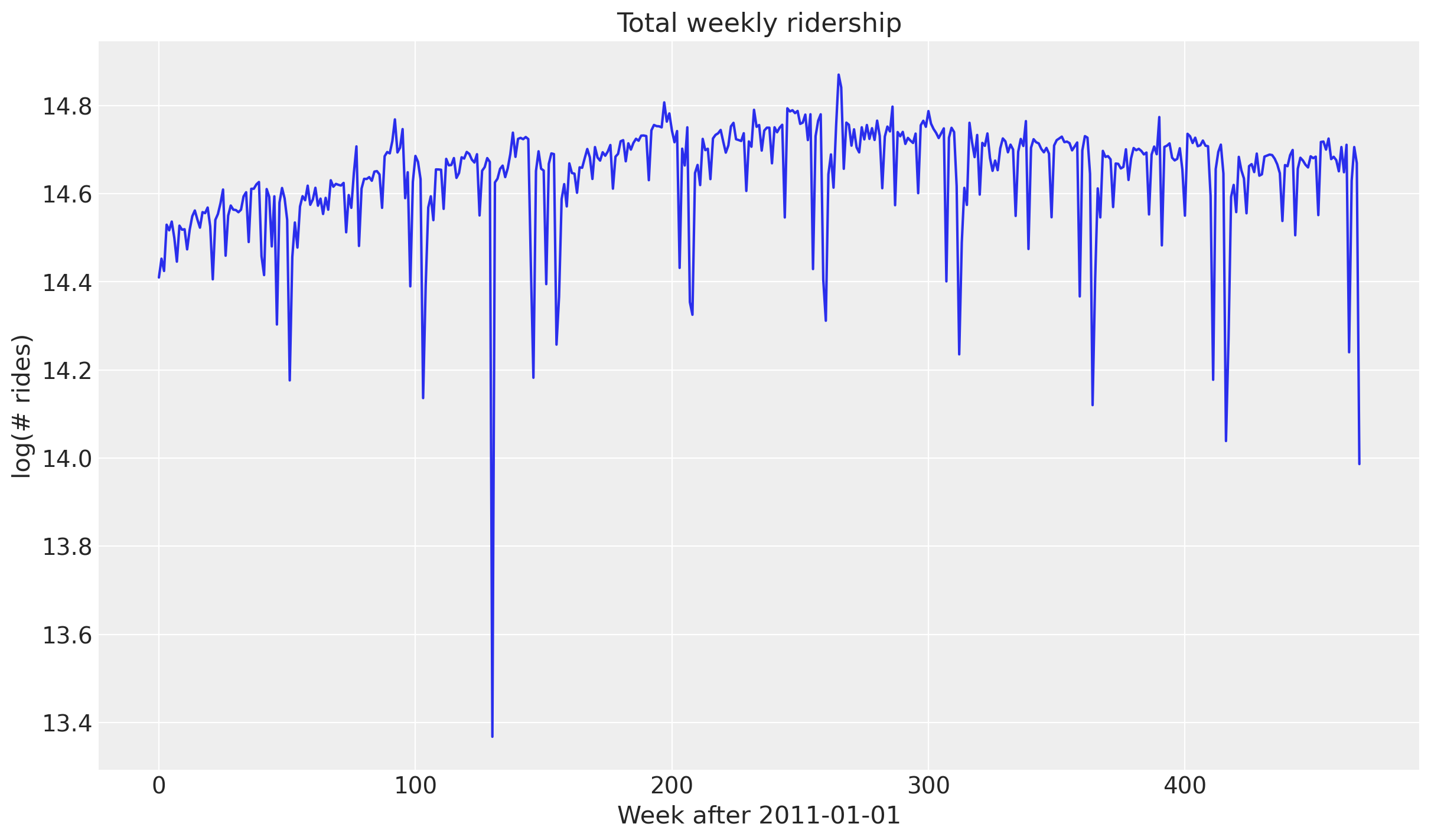
“Consider a simple univariate dataset, say weekly BART train ridership aggregated over all stations in the network.”
dataset = load_bart_od()
print(dataset.keys())
print(dataset["counts"].shape)
print(" ".join(dataset["stations"]))
dict_keys(['stations', 'start_date', 'counts'])
torch.Size([78888, 50, 50])
12TH 16TH 19TH 24TH ANTC ASHB BALB BAYF BERY CAST CIVC COLM COLS CONC DALY DBRK DELN DUBL EMBR FRMT FTVL GLEN HAYW LAFY LAKE MCAR MLBR MLPT MONT NBRK NCON OAKL ORIN PCTR PHIL PITT PLZA POWL RICH ROCK SANL SBRN SFIA SHAY SSAN UCTY WARM WCRK WDUB WOAK“This data roughly logarithmic, so we log-transform for modeling.”
T, _, _ = dataset["counts"].shape
data = (
    dataset["counts"][: T // (24 * 7) * 24 * 7].reshape(T // (24 * 7), -1).sum(-1).log()
)
data = data.unsqueeze(-1)
# We convert the Torch tensor to a JAX array
data = jnp.array(data)
Let’s plot the data.
fig, ax = plt.subplots()
ax.plot(data)
ax.set(
    title="Total weekly ridership",
    ylabel="log(# rides)",
    xlabel="Week after 2011-01-01",
);
Split Data
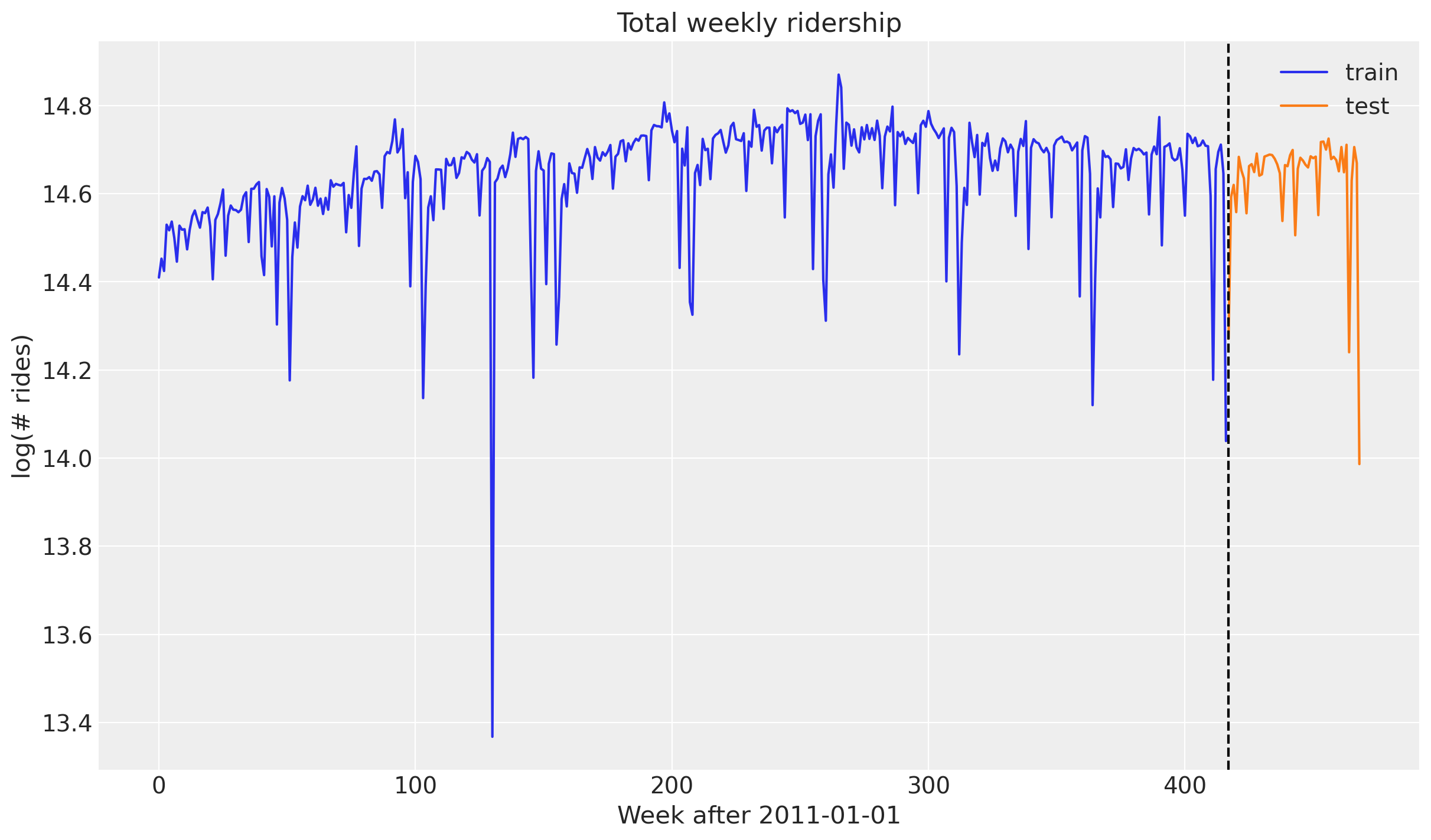
We do a train/test split leaving the last year for testing.
T0 = 0  # beginning
T2 = data.shape[-2]  # end
T1 = T2 - 52  # train/test split

y_train = data[T0:T1]
y_test = data[T1:T2]

print(f"data_train shape: {y_train.shape}")
print(f"data_test shape: {y_test.shape}")
data_train shape: (417, 1)
data_test shape: (52, 1)fig, ax = plt.subplots()
ax.plot(jnp.arange(T1), y_train, label="train")
ax.plot(jnp.arange(T1, T2), y_test, label="test")
ax.axvline(T1, c="black", linestyle="--")
ax.legend()
ax.set(
title="Total weekly ridership",
ylabel="log(# rides)",
xlabel="Week after 2011-01-01",
);
Seasonal Features
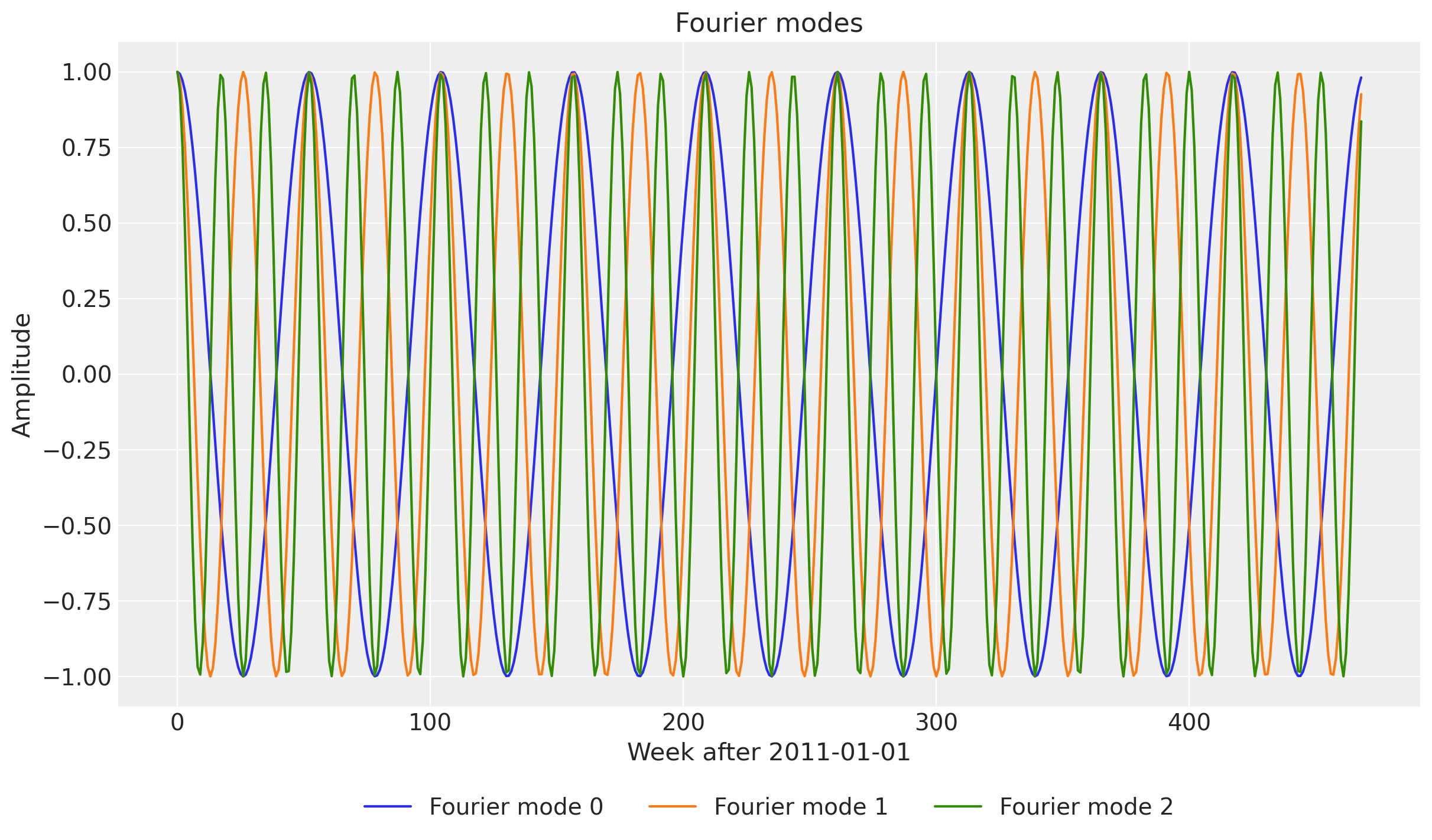
We will describe the model specification below. One key feature in the final Pyro model is the use of Fourier features to model the seasonal component.
We can generate the Fourier features using the periodic_features function from Pyro.
“When also
min_periodis specified this generates periodic features at large length scales, but omits high frequency features.”
fourier_modes_torch = periodic_features(duration=T2, max_period=365.25 / 7)

fourier_modes_torch.shape
torch.Size([469, 52])The first dimension is the time component and the second dimension is the Fourier features. In this case we have \(52\) terms. Let’s look into the first few Fourier features.
fig, ax = plt.subplots()
for i in range(3):
    ax.plot(fourier_modes_torch[:, i], label=f"Fourier mode {i}")
ax.legend(loc="lower center", bbox_to_anchor=(0.5, -0.2), ncol=3)
ax.set(
    title="Fourier modes",
    ylabel="Amplitude",
    xlabel="Week after 2011-01-01",
);
Now, let’s (try to) look into all of them.
fig, ax = plt.subplots()
ax.plot(fourier_modes_torch, color="C0", alpha=0.02)
ax.set(
    title="Fourier modes",
    ylabel="Amplitude",
    xlabel="Week after 2011-01-01",
);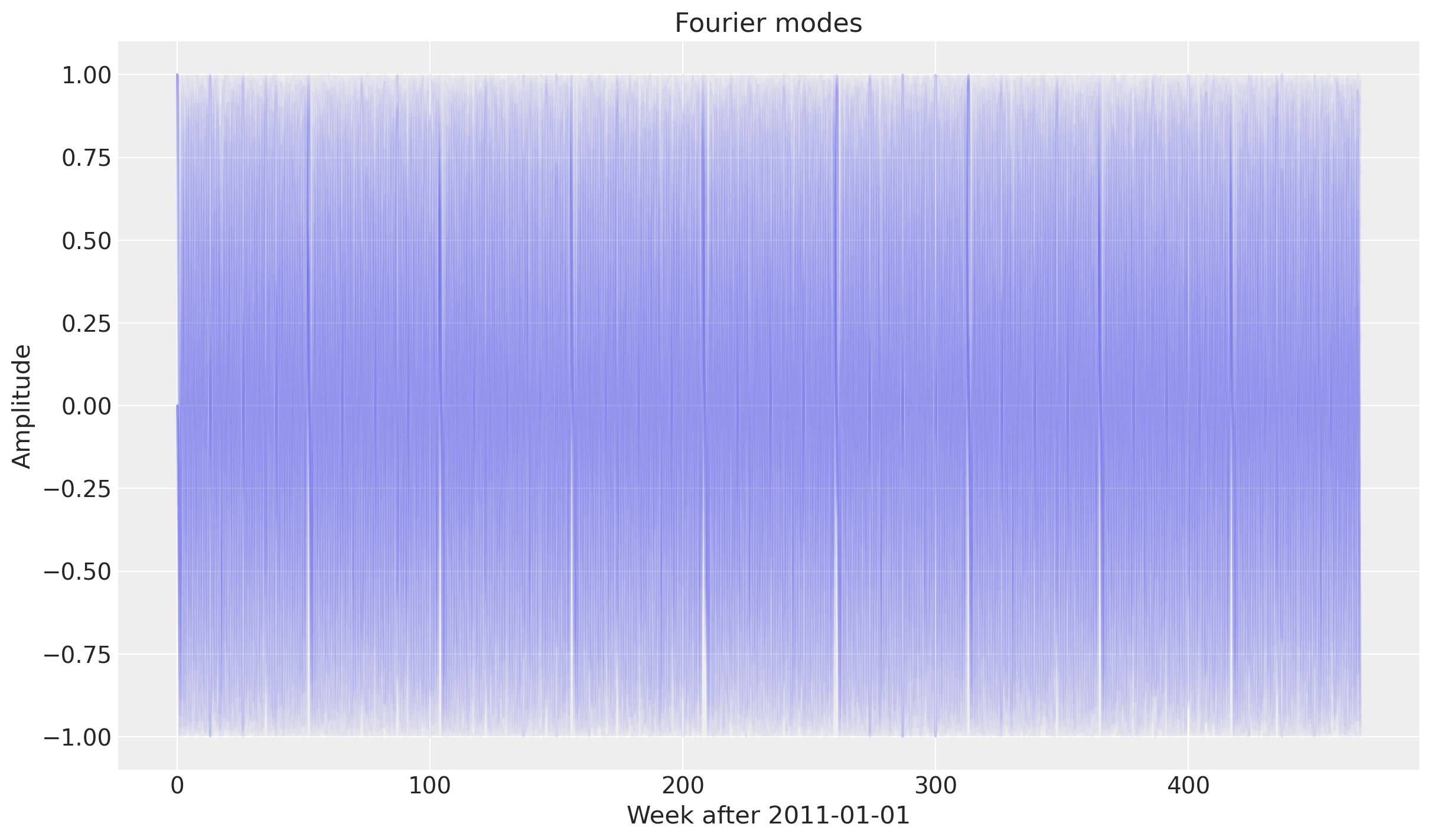
These are enough features to model the seasonality at different frequencies.
For illustration purposes, let’s implement the same function in NumPyro.
def periodic_features_jax(
    duration: int,
    max_period: float | None = None,
    min_period: float | None = None,
    **options: Any,
) -> Float[Array, "t_max feature_dim"]:
    assert isinstance(duration, int) and duration >= 0
    if max_period is None:
        max_period = duration
    if min_period is None:
        min_period = 2
    assert min_period >= 2, "min_period is below Nyquist cutoff"
    assert min_period <= max_period

    t = jnp.arange(float(duration), **options).reshape(-1, 1, 1)
    phase = jnp.array([0, jnp.pi / 2], **options).reshape(1, -1, 1)
    freq = jnp.arange(1, max_period / min_period, **options).reshape(1, 1, -1) * (
        2 * jnp.pi / max_period
    )
    return jnp.cos(freq * t + phase).reshape(duration, -1)


# Generate Fourier Features in JAX
fourier_modes_jax = periodic_features_jax(T2, 365.25 / 7)
# Verify that the Fourier features are the same as the Pyro code
assert jnp.allclose(jnp.array(fourier_modes_torch), fourier_modes_jax)
Train - Test Split
Next, we split these features into train and test.
time = jnp.arange(T2)
time_train = time[:T1]
time_test = time[T1:T2]

fourier_modes_train = fourier_modes_jax[:T1]
fourier_modes_test = fourier_modes_jax[T1:T2]

print(
    f"""
    time_train shape: {time_train.shape}
    time_test shape: {time_test.shape}
    ---
    fourier_modes_train shape: {fourier_modes_train.shape}
    fourier_modes_test shape: {fourier_modes_test.shape}
"""
)
time_train shape: (417,)
time_test shape: (52,)
---
fourier_modes_train shape: (417, 52)
fourier_modes_test shape: (52, 52)Finally, we store these features in a single array (in other models we can keep adding features to this covariates array).
covariates = fourier_modes_jax

covariates_train = covariates[:T1]
covariates_test = covariates[T1:T2]

print(f"covariates_train shape: {covariates_train.shape}")
print(f"covariates_test shape: {covariates_test.shape}")
covariates_train shape: (417, 52)
covariates_test shape: (52, 52)Model Specification
To forecast the data, we will use a local level model with a seasonal component. The model is the following:
\[ y_t = \text{bias} + \mu_t + \text{weight} \times \text{covariates} + \varepsilon_t \]
where:
- \(\mu_t \sim \text{Normal}(\mu_{t-1}, \text{drift_scale})\) with \(\mu_0 = 0\)
- \(\varepsilon_t \sim \text{StudentT}(\nu, 0, \sigma)\)
Here are some additional observations about the model:
- We use the same priors as the Pyro example.
- We use the
scanhandler to efficiently compute the latent levels \(\mu_t\). for this case it is not strictly necessary as we could use a simple cumulative sum, but is a nice addition as this is a very common pattern in time series models with NumPyro. See for example Notes on Exponential Smoothing with NumPyro - We use the
LocScaleReparamto reparameterize the drift. In this example, this helps the inference with stochastic variational inference (SVI) quite a lot!. Moreover, we learn the parametrization level (from centered to non-centered) as part of the inference process.
Let’s see the model specification.
def model(
    covariates: Float[Array, "t_max feature_dim"],
    y: Float[Array, "t_max n_series"] | None = None,
) -> None:
    # Get the time and feature dimensions
    t_max, feature_dim = covariates.shape
    # Sample the bias (intercept)
    bias = numpyro.sample("bias", dist.Normal(loc=0, scale=10))
    # Sample the weight (regression coefficients for the covariates)
    weight = numpyro.sample(
        "weight", dist.Normal(loc=0, scale=0.1).expand([feature_dim]).to_event(1)
    )

    # Global scale for the drift
    drift_scale = numpyro.sample("drift_scale", dist.LogNormal(loc=-20, scale=5))

    # Degrees of freedom for the Student-T distribution
    nu = numpyro.sample("nu", dist.Gamma(concentration=10, rate=2))
    # Scale for the Student-T distribution
    sigma = numpyro.sample("sigma", dist.LogNormal(loc=-5, scale=5))

    # Sample the centered parameter for the LocScaleReparam
    centered = numpyro.sample("centered", dist.Uniform(low=0, high=1))

    with (
        numpyro.plate("time", t_max),
        numpyro.handlers.reparam(config={"drift": LocScaleReparam(centered=centered)}),
    ):
        drift = numpyro.sample("drift", dist.Normal(loc=0, scale=drift_scale))

    def transition_fn(carry, t):
        "Local level transition function"
        previous_level = carry
        current_level = previous_level + drift[t]
        return current_level, current_level

    # Compute the latent levels using scan
    _, pred_levels = scan(transition_fn, init=jnp.zeros((1,)), xs=jnp.arange(t_max))

    # Compute the mean of the model
    mu = pred_levels + bias + (weight * covariates).sum(axis=-1, keepdims=True)

    # Sample the observations
    with numpyro.handlers.condition(data={"obs": y}):
        numpyro.sample("obs", dist.StudentT(df=nu, loc=mu, scale=sigma))
We can visualize the model structure.
numpyro.render_model(
    model=model,
    model_kwargs={
        "covariates": covariates_train,
        "y": y_train,
    },
    render_distributions=True,
    render_params=True,
)
Prior Predictive Check
Before we start the inference, let’s see what the model prior predictive looks like.
prior_predictive = Predictive(model=model, num_samples=2_000, return_sites=["obs"])

rng_key, rng_subkey = random.split(rng_key)

prior_samples = prior_predictive(rng_subkey, covariates_train)

idata_prior = az.from_dict(
    prior_predictive={k: v.transpose(2, 0, 1) for k, v in prior_samples.items()},
    coords={"time_train": time_train},
    dims={"obs": ["time_train"]},
)
fig, ax = plt.subplots()
for hdi_prob in [0.50, 0.94]:
az.plot_hdi(
jnp.arange(T1),
idata_prior["prior_predictive"]["obs"],
hdi_prob=hdi_prob,
color="C0",
fill_kwargs={
"alpha": 0.3,
"label": f"{hdi_prob*100:.0f}% HDI train",
},
smooth=False,
ax=ax,
)
ax.plot(jnp.arange(T1), y_train, label="train")
ax.legend(loc="lower center", bbox_to_anchor=(0.5, -0.2), ncol=3)
ax.set(
title="Prior predictive",
ylabel="log(# rides)",
xlabel="Week after 2011-01-01",
)
fig.suptitle("Total weekly ridership", fontsize=18, fontweight="bold");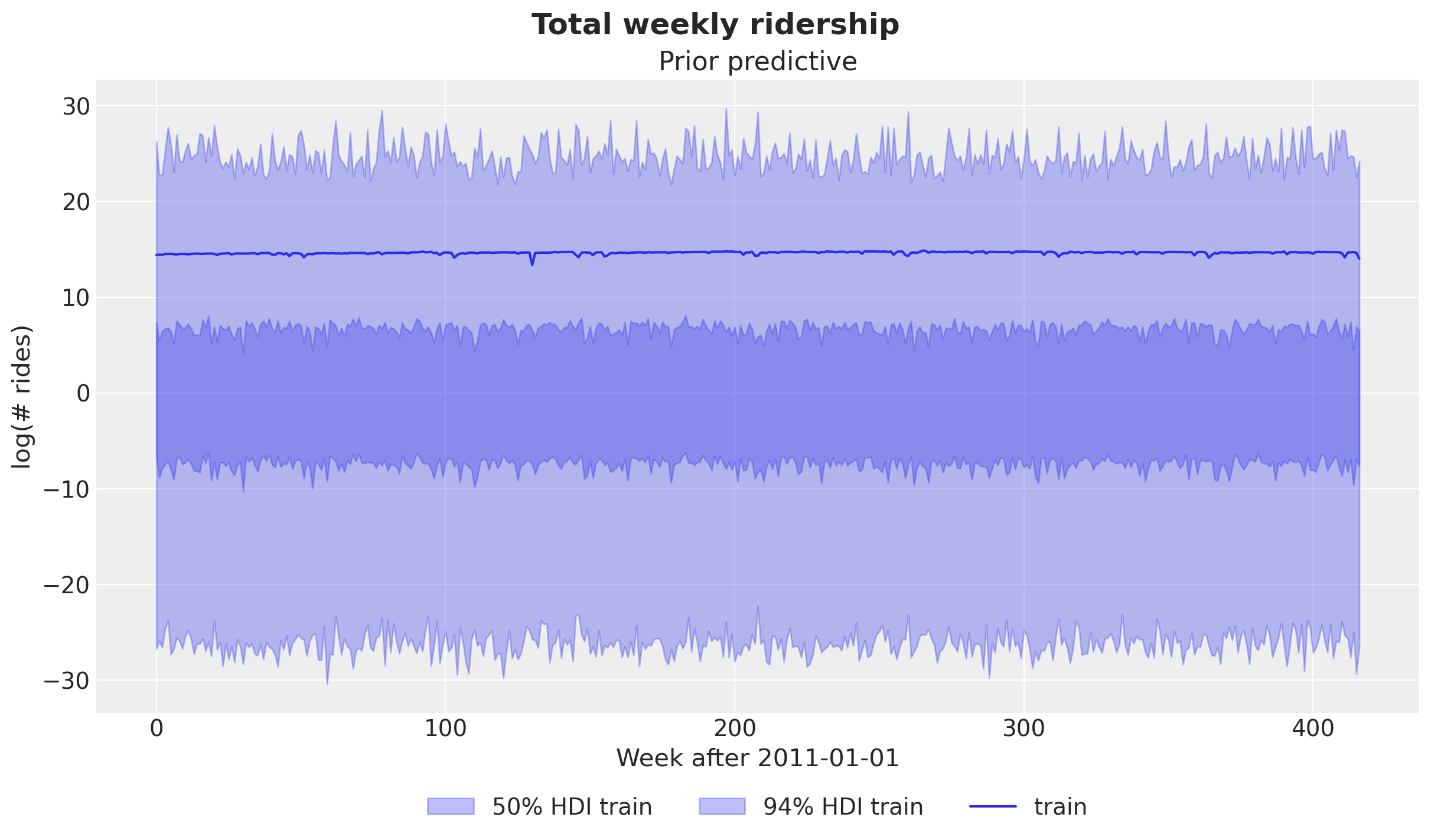
The priors are not very informative (we can do a bit better, for example specifying a narrower range for the bias), but overall the prior samples look within a reasonable range.
Inference with SVI
Now we proceed to run the inference using SVI.
%%time

guide = AutoNormal(model)
optimizer = numpyro.optim.Adam(step_size=0.005)
svi = SVI(model, guide, optimizer, loss=Trace_ELBO())
num_steps = 50_000

rng_key, rng_subkey = random.split(key=rng_key)

svi_result = svi.run(
    rng_subkey,
    num_steps,
    covariates_train,
    y_train,
)

fig, ax = plt.subplots(figsize=(9, 6))
ax.plot(svi_result.losses)
ax.set_title("ELBO loss", fontsize=18, fontweight="bold");
100%|██████████| 50000/50000 [00:10<00:00, 4756.01it/s, init loss: 5835.2622, avg. loss [47501-50000]: -421.0681]
CPU times: user 13.6 s, sys: 693 ms, total: 14.3 s
Wall time: 13.8 s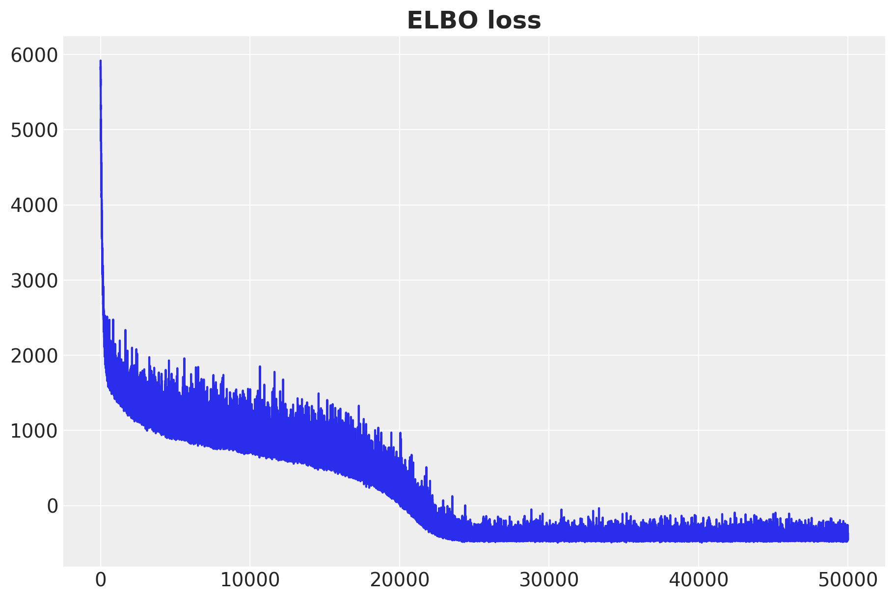
The ELBO loss is decreasing as expected.
Posterior Predictive Check
We can use the fitted model to sample from the posterior predictive distribution and generate posterior samples for the train and test data.
posterior = Predictive(
    model=model,
    guide=guide,
    params=svi_result.params,
    num_samples=5_000,
    return_sites=["obs"],
)
rng_key, rng_subkey = random.split(rng_key)
idata_train = az.from_dict(
posterior_predictive={
k: v.transpose(2, 0, 1)
for k, v in posterior(rng_subkey, covariates_train).items()
},
coords={"time_train": time_train},
dims={"obs": ["time_train"]},
)
idata_test = az.from_dict(
posterior_predictive={
k: v.transpose(2, 0, 1) for k, v in posterior(rng_subkey, covariates).items()
},
coords={"time": time},
dims={"obs": ["time"]},
)Model Evaluation
Before looking into the predictions, let’s specify the evaluation metric beforehand. We will use the Continuous Ranked Probability Score (CRPS) to evaluate the performance of the model. This is a very common metric for probabilistic forecasting models (see for example Hierarchical Exponential Smoothing Model). It serves as a generalization of the mean absolute error to probabilistic models. A summarized description of the CRPS is the following (from CRPS — A Scoring Function for Bayesian Machine Learning Models)
“The CRPS — Continuous Ranked Probability Score — is a score function that compares a single ground truth value to a Cumulative Distribution Function. It t can be used as a metric to evaluate a model’s performance when the target variable is continuous and the model predicts the target’s distribution; Examples include Bayesian Regression or Bayesian Time Series models.”
Pyro offers a function pyro.ops.stats.crps_empirical to compute the CRPS, but we will write our own using JAX to better understand the underlying computation.
def crps(
    truth: Float[Array, "t_max n_series"],
    pred: Float[Array, "n_samples t_max n_series"],
    sample_weight: Float[Array, " t_max"] | None = None,
) -> Float[Array, ""]:
    if pred.shape[1:] != (1,) * (pred.ndim - truth.ndim - 1) + truth.shape:
        raise ValueError(
            f"""Expected pred to have one extra sample dim on left.
            Actual shapes: {pred.shape} versus {truth.shape}"""
        )

    absolute_error = jnp.mean(jnp.abs(pred - truth), axis=0)

    num_samples = pred.shape[0]
    if num_samples == 1:
        return jnp.average(absolute_error, weights=sample_weight)

    pred = jnp.sort(pred, axis=0)
    diff = pred[1:] - pred[:-1]
    weight = jnp.arange(1, num_samples) * jnp.arange(num_samples - 1, 0, -1)
    weight = weight.reshape(weight.shape + (1,) * (diff.ndim - 1))

    per_obs_crps = absolute_error - jnp.sum(diff * weight, axis=0) / num_samples**2
    return jnp.average(per_obs_crps, weights=sample_weight)


crps_train = crps(
    y_train,
    jnp.array(
        idata_train["posterior_predictive"]["obs"]
        .transpose(..., "time_train", "chain")
        .to_numpy()
    ),
)

crps_test = crps(
    y_test,
    jnp.array(
        idata_test["posterior_predictive"]["obs"][:, :, T1:T2]
        .transpose(..., "time", "chain")
        .to_numpy()
    ),
)
Let’s plot the posterior predictive samples forecast of the train and test sets.
fig, ax = plt.subplots()

for i, hdi_prob in enumerate([0.94, 0.5]):
    az.plot_hdi(
        time_train,
        idata_train["posterior_predictive"]["obs"],
        hdi_prob=hdi_prob,
        color="C0",
        fill_kwargs={
            "alpha": 0.3 + 0.1 * i,
            "label": f"{hdi_prob*100:.0f}% HDI train",
        },
        smooth=False,
        ax=ax,
    )
    az.plot_hdi(
        time_test,
        idata_test["posterior_predictive"]["obs"][:, :, T1:T2],
        hdi_prob=hdi_prob,
        color="C1",
        fill_kwargs={
            "alpha": 0.3 + 0.1 * i,
            "label": f"{hdi_prob*100:.0f}% HDI test",
        },
        smooth=False,
        ax=ax,
    )

ax.plot(jnp.arange(T1), y_train, label="train")
ax.plot(jnp.arange(T1, T2), y_test, label="test")
ax.axvline(T1, c="black", linestyle="--")
ax.legend(loc="lower center", bbox_to_anchor=(0.5, -0.3), ncol=3)
ax.set(
    title=f"Train CRPS: {crps_train:.4f} | Test CRPS: {crps_test:.4f}",
    ylabel="log(# rides)",
    xlabel="Week after 2011-01-01",
)
fig.suptitle("Total weekly ridership", fontsize=18, fontweight="bold");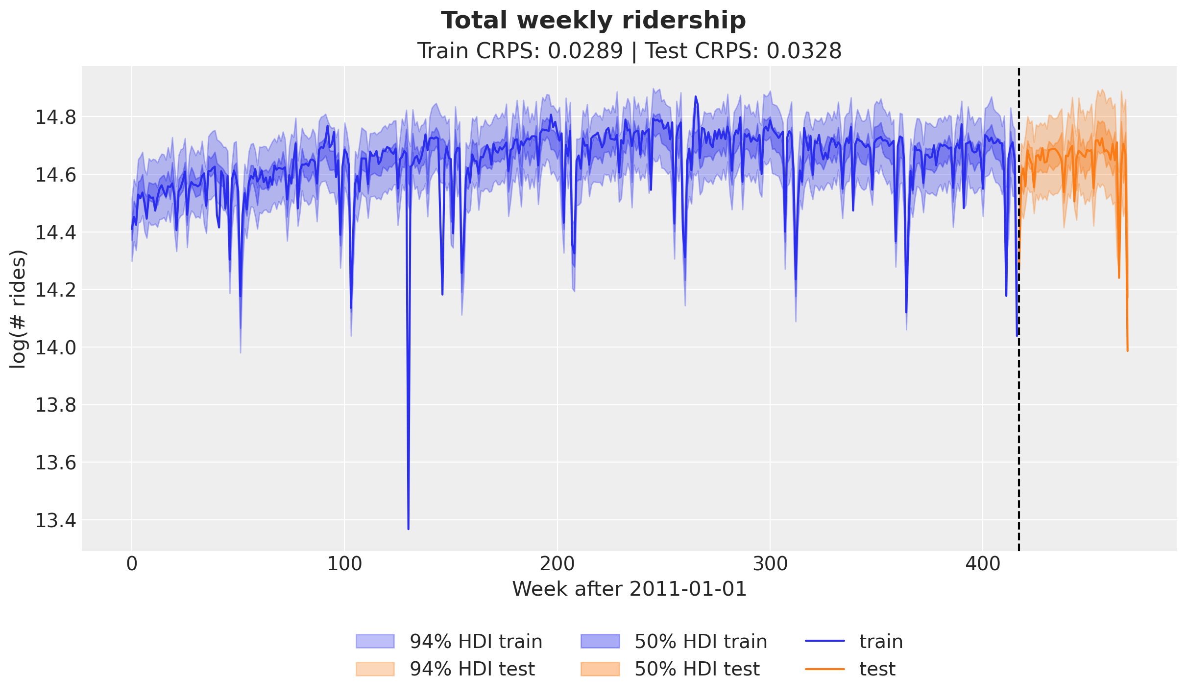
Overall, the in sample and out of sample prediction look good! The CRPS values are comparable to the ones reported in the Pyro example.
Finally, let’s plot the posterior predictive mean for the test set.
fig, ax = plt.subplots()

for i, hdi_prob in enumerate([0.94, 0.5]):
    az.plot_hdi(
        jnp.arange(T1, T2),
        idata_test["posterior_predictive"]["obs"][:, :, T1:T2],
        hdi_prob=hdi_prob,
        color="C1",
        fill_kwargs={
            "alpha": 0.3 + 0.1 * i,
            "label": f"{hdi_prob*100:.0f}% HDI test",
        },
        smooth=False,
        ax=ax,
    )

ax.plot(
    time_test,
    idata_test["posterior_predictive"]["obs"][:, :, T1:T2].mean(dim=("chain", "draw")),
    marker="o",
    color="C1",
    label="posterior predictive mean",
)
ax.plot(jnp.arange(T1, T2), y_test, marker="o", color="black", label="test")
ax.legend(loc="lower center", bbox_to_anchor=(0.5, -0.2), ncol=4)
ax.set(
    title=f"Test CRPS: {crps_test:.4f}",
    ylabel="log(# rides)",
    xlabel="Week after 2011-01-01",
)
fig.suptitle("Total weekly ridership (test set)", fontsize=18, fontweight="bold");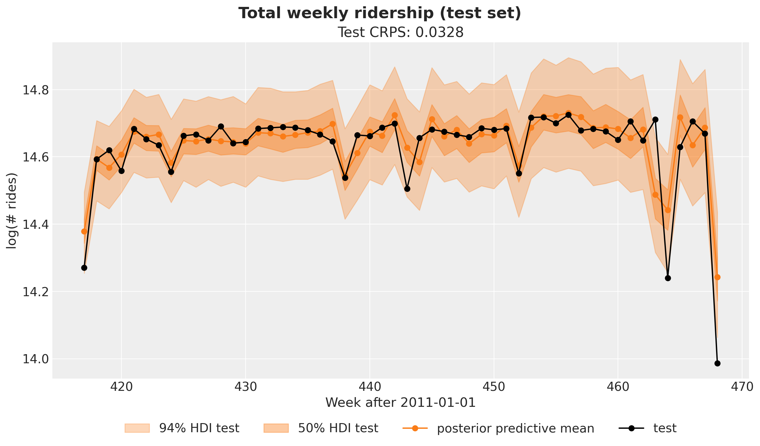
Next Steps
We could modularize the whole forecasting fitting and evaluation process to be able to run a time-slice cross-validation analysis. Pyro offers great tooling to do this.