In this post I want to describe how to sample from a multivariate normal distribution following section A.2 Gaussian Identities of the book Gaussian Processes for Machine Learning. This is a first step towards exploring and understanding Gaussian Processes methods in machine learning.

Multivariate Normal Distribution

Recall that a random vector \(X = (X_1, , X_d)\) has a multivariate normal (or Gaussian) distribution if every linear combination

\[ \sum_{i=1}^{d} a_iX_i, \quad a_i\in\mathbb{R} \] is normally distributed.

Warning: The sum of two normally distributed random variables does not need to be normally distributed (see below).

The multivariate normal distribution has a joint probability density given by

\[ p(x|m,K_0) =(2\pi)^{−d/2}|K_0|^{−1/2}\exp\left(-\frac{1}{2}(x−m)^T {K_0}^{-1}(x−m)\right), \]

where \(m ^d\) is the mean vector and \(K_0 M_d() \) is the (symmetric, positive definite) covariance matrix.

Prepare Notebook

import numpy as np 
import matplotlib.pyplot as plt
import seaborn as sns; sns.set()

Set Parameters

# Define dimension. 
d = 2

# Set mean vector. 
m = np.array([1, 2]).reshape(2, 1)

# Set covariance function. 
K_0 = np.array([[2, 1],
                [1, 2]])

Let us compute the eigenvalues of \(K_0\).

# Eigenvalues covariance function.
np.linalg.eigvals(K_0)

array([3., 1.])

We see that \(K_0\) is indeed positive definite (see The Spectral Theorem for Matrices).

Sampling Process

Step 1: Compute the Cholesky Decomposition

We want to compute the Cholesky decomposition of the covariance matrix \(K_0\). That is, we want to find a lower triangular matrix \(LM_d()\) such that \(K_0 = LL^T\).

“In practice it may be necessary to add a small multiple of the identity matrix \(I\) to the covariance matrix for numerical reasons. This is because the eigenvalues of the matrix \(K_0\) can decay very rapidly and without this stabilization the Cholesky decomposition fails. The effect on the generated samples is to add additional independent noise of variance \(\). From the context \(\) can usually be chosen to have inconsequential effects on the samples, while ensuring numerical stability.” (A.2 Gaussian Identities)

# Define epsilon.
epsilon = 0.0001

# Add small pertturbation. 
K = K_0 + epsilon*np.identity(d)

#  Cholesky decomposition.
L = np.linalg.cholesky(K)
L

array([[1.41424892, 0.        ],
       [0.7070891 , 1.2247959 ]])

Let us verify the desired property:

np.dot(L, np.transpose(L))

array([[2.0001, 1.    ],
       [1.    , 2.0001]])

Step 2: Generate Independent Samples \(u ∼ N(0,I)\)

# Number of samples. 
n = 10000

u = np.random.normal(loc=0, scale=1, size=d*n).reshape(d, n)

Step 3: Compute \( x = m + Lu \)

The variable \( x = m + Lu \) has a multivariate normal distribution since is a linear combination of independent normally distributed variables. Moreover,

\[ E[x] = E[m + Lu] = m + LE[u] = m \]

and

\[ E[xx^T] = E[mm^T] + E[mu^TL^T] + E[Lum^T] + E[Luu^TL^T] = ||m^2|| + LE[uu^T]L^T = \lVert m \rVert^2 + K \]

hence, \(E[(x-m)(x^T-mT)] = K\).

x = m + np.dot(L, u)

Plot Distribution

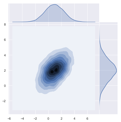
Let us plot the density function.

sns.jointplot(x=x[0], y=x[1], kind="kde", space=0);

Using Numpy Sampler

Numpy has a build in multivariate normal sampling function:

z = np.random.multivariate_normal(mean=m.reshape(d,), cov=K, size=n)

y = np.transpose(z)

# Plot density function.
sns.jointplot(x=y[0], y=y[1], kind="kde", space=0);

Sums of Normal Random Variables need not be Normal

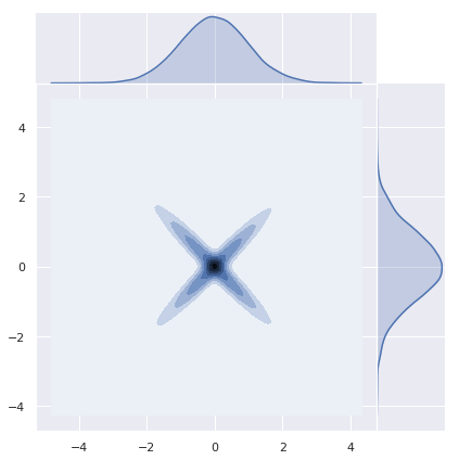
As an important remark, note that sums of normal random variables need not be normal. Let us see a concrete example studied in detail here. Let \(Z_1 N(0,1)\) and define \(Z_2 := (Z_1)Z_1\). Then, \(Z_1 + Z_2\) is not normally distributed.

z_1 = np.random.normal(loc=0, scale=1, size=n)
z = np.random.normal(loc=0, scale=1, size=n)

z_2 = np.sign(z)*z_1

sns.jointplot(x=z_1, y=z_2, kind="kde", space=0);

Sampling from a Multivariate Normal Distribution