In this post I want to present some \(\LaTeX\) code to create common manifold figures which I often used during my graduate studies in differential geometry. I am going to use the TikZ package. In this short paper there is a brief introduction to this package.
I am going to describe the structure of the .tex file. Let us first define the document type and load the TikZ package.
\documentclass[11pt]{amsart}
\usepackage{tikz}
Next we begin the document.
\begin{document}Cylinder
We draw a schematic picture of a cylinder on a closed manifold \(N\).
\begin{tikzpicture}
\draw[rounded corners=35pt](0,0)--(8,0);
\draw[rounded corners=35pt](0,-2)--(8,-2);
\draw (8.5,-1) arc (0:360:0.5cm and 1cm);
\draw (0.5,-1) arc (0:360:0.5cm and 1cm);
\node (a) at (0,0.5) {$N$};
\node (b) at (4,-2.5) {$\mathbb{R}^+$};
\end{tikzpicture}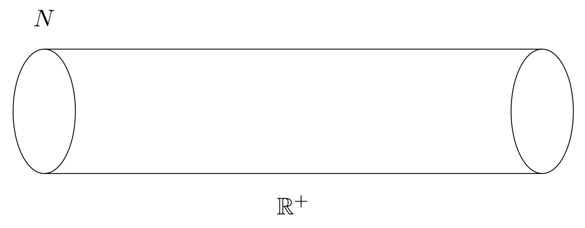
Manifold with Boundary
\begin{tikzpicture}
\draw[rounded corners=35pt](7,-1)--(4.2,-1)--(2,-2)--(0,0) -- (2,2)--(4.2,1)--(7,1);
\draw (1.5,0.2) arc (175:315:1cm and 0.5cm);
\draw (3,-0.28) arc (-30:180:0.7cm and 0.3cm);
\draw (7.5,0) arc (0:360:0.5cm and 1cm);
\node (a) at (20:2.5) {$M$};
\node (a) at (-12:7.5) {$\partial M=N$};
\end{tikzpicture}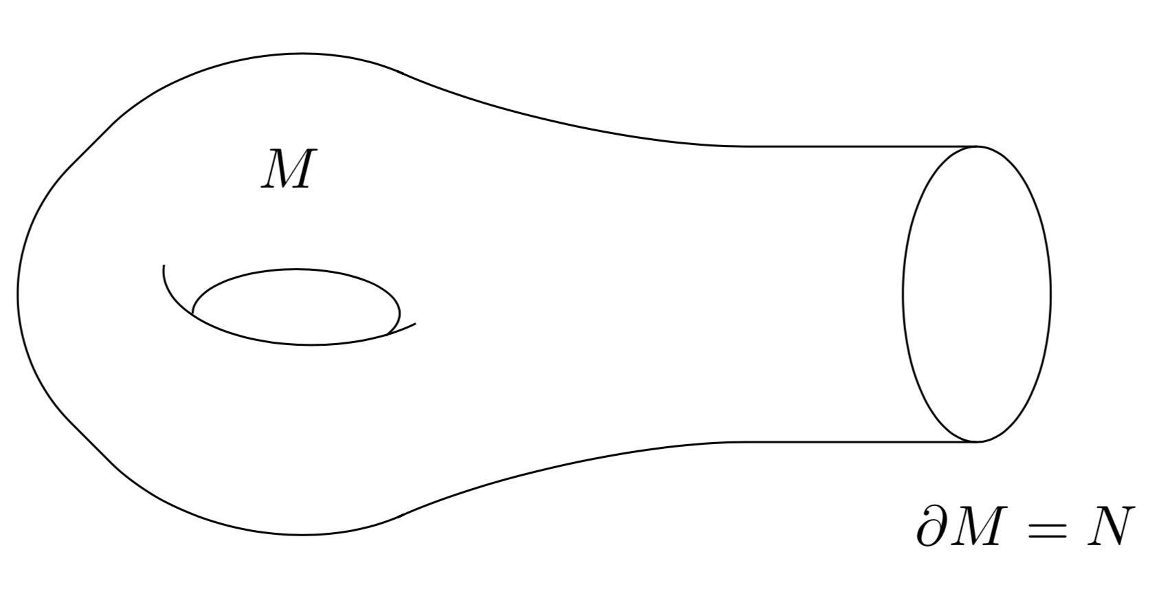
Manifold with Boundary + Cylinder
In geometric analysis it is quite common to attach a cylinder to a manifold with boundary (\(L^2\)-index theorems).
\begin{tikzpicture}
\draw[rounded corners=35pt](7.5,-1)--(4.2,-1)--(2,-2)--(0,0) -- (2,2)--(4.2,1)--(7.5,1);
\draw (1.5,0.2) arc (175:315:1cm and 0.5cm);
\draw (3,-0.28) arc (-30:180:0.7cm and 0.3cm);
\draw (6,0) arc (0:360:0.5cm and 1cm);
\draw (8,0) arc (0:360:0.5cm and 1cm);
\node (a) at (20:2.5) {$M$};
\node (a) at (12:6.5) {$[0,1]$};
\node (a) at (-12:7.5) {$\partial M$};
\end{tikzpicture}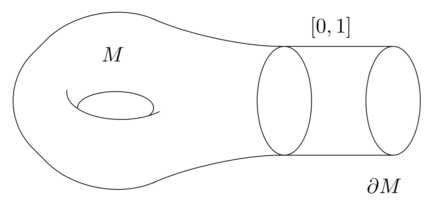
Double Manifold
The double \(\tilde{M}\) of a manifold with boundary \(M\) is the resulting closed manifold obtained by gluing two copies of \(M\) along the boundary. Concretely, \(\tilde{M} = M \cup (- M)\), where \(-M\) denotes \(M\) with the orientation reversed.
\begin{tikzpicture}
\draw[rounded corners=35pt](6,-1)--(4.2,-1)--(2,-2)--(0,0)--(2,2)--(4.2,1)--(7,1)--(9.2,2)--(11,0)
--(9,-2)--(6,-1);
\draw (1.5,0.2) arc (175:315:1cm and 0.5cm);
\draw (3,-0.28) arc (-30:180:0.7cm and 0.3cm);
\draw (5.8,0) arc (0:360:0.5cm and 1cm);
\draw (7.5,0.2) arc (175:315:1cm and 0.5cm);
\draw (9,-0.28) arc (-30:180:0.7cm and 0.3cm);
\node (a) at (-13:5.8) {$\partial M$};
\node (a) at (26:2.5) {$\tilde{M}$};
\end{tikzpicture}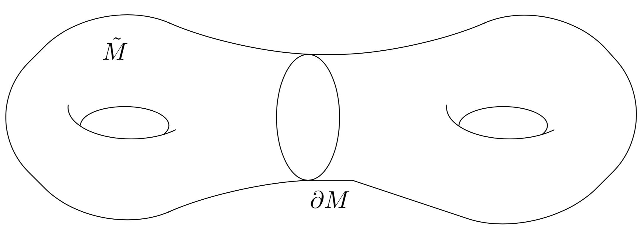
Cobordant Manifolds
The following is the most common schematic figure of cobordant manifolds.
\begin{figure}[h]
\begin{center}
\begin{tikzpicture}
\draw[rounded corners=50pt](0,2)--(3,0)--(0,-2);
\draw (0.3,2.7) arc (0:360:0.3 and 0.7);
\draw [->>] (0.3,-2.7) arc (0:360:0.3 and 0.7);
\draw[rounded corners=50pt](0,3.4)--(4,1)--(7,1);
\draw[rounded corners=50pt](0,-3.4)--(4,-1)--(7,-1);
\draw [->>](7.3,0) arc (0:360:0.3 and 1);
\draw (3.5,0.2) arc (175:315:1cm and 0.5cm);
\draw (5,-0.28) arc (-30:180:0.7cm and 0.3cm);
\end{tikzpicture}
\caption{Two cobordant manifolds,}
\end{center}
\end{figure}
Finally, we end the document.
\end{document}