Introduction to R Plumber : Expose a Caret model to a web API

In this post we explore the basics of the Plumber package. Our aim is to ilustrate how to fit a \(L^2\)-regularized linear model and expose it to a web API so that we can request predictions.

Prepare Notebook

Let us load the necessary libraries.

library(caret)
library(httr)
library(magrittr)
library(plumber)
library(tidyverse)

Load Data

As a toy example we consider the mtcars data set.

df <- mtcars %>% as_tibble()

df %>% head

## # A tibble: 6 x 11
##     mpg   cyl  disp    hp  drat    wt  qsec    vs    am  gear  carb
##   <dbl> <dbl> <dbl> <dbl> <dbl> <dbl> <dbl> <dbl> <dbl> <dbl> <dbl>
## 1  21       6   160   110  3.9   2.62  16.5     0     1     4     4
## 2  21       6   160   110  3.9   2.88  17.0     0     1     4     4
## 3  22.8     4   108    93  3.85  2.32  18.6     1     1     4     1
## 4  21.4     6   258   110  3.08  3.22  19.4     1     0     3     1
## 5  18.7     8   360   175  3.15  3.44  17.0     0     0     3     2
## 6  18.1     6   225   105  2.76  3.46  20.2     1     0     3     1

We want to fit a simple linear model to predict the variable mpg.

Warning: We are not interested to find the “best model”. Better feature engineering and hyperparameter tunig is not developed here because it is not the main purpose.

Correlation Plot

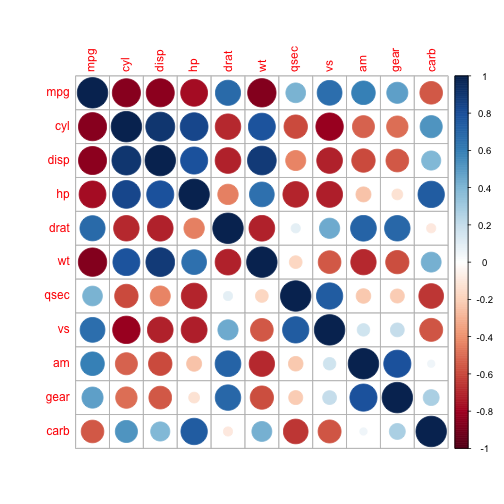
For variable selection we consider a correlation plot.

df %>% cor %>% corrplot::corrplot()

From the visualization we see that the variables wt, qsec and am could be good predictors.

Define and Train Model

We are going to use the Caret package.

Split Data

set.seed(seed = 0)

# Define observation matrix. 
X <- df %>% select(wt, qsec, am)
# Define target vector.
y <- df %>% pull(mpg)

# Define a partition of the data. 
partition <- createDataPartition(y = y, p = 0.75, list = FALSE) 

# Split the data into a training and test set. 
df.train <- df[partition, ]
df.test <- df[- partition, ]

X.train <- df.train %>% select(wt, qsec, am)
y.train <- df.train %>% pull(mpg)

X.test <- df.test %>% select(wt, qsec, am)
y.test <- df.test %>% pull(mpg)

Data Pre-Processing

As we want to use a linear model, we neet to scale the variables.

# Define scaler object. 
scaler.obj <- preProcess(x = X.train, method = c('center', 'scale'))

# Transform the data. 
X.train.scaled <- predict(object = scaler.obj, newdata = X.train)
X.test.scaled <- predict(object = scaler.obj, newdata = X.test)

Train Model

We fit \(L^2\)-regularization linear model using a 3-fold cross-validation to tune the regularization hyperparameter.

model.obj <-  train(x = X.train.scaled,
                    y = y.train,
                    method = 'ridge',
                    trControl = trainControl(method = 'cv', number = 3), 
                    metric = 'RMSE')

Model Evaluation

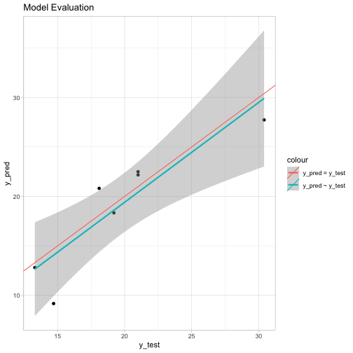
Let us evaluate the model perforance.

On the training set:

model.obj$results %>% select(RMSE)

##       RMSE
## 1 2.613844
## 2 2.613700
## 3 2.554912

On the test set:

y.pred <- predict(model.obj, newdata = X.test.scaled)

RMSE(pred = y.pred, obs = y.test)

## [1] 2.664047

The model seems to be stable and there is no strong evidence of overfitting.

Visualization

tibble(y_test = y.test, y_pred = y.pred) %>% 
  ggplot() + 
  theme_light() + 
  geom_point(mapping = aes(x = y_test, y = y_pred)) + 
  geom_smooth(mapping = aes(x = y_test, y = y_pred, colour = 'y_pred ~ y_test'), method = 'lm', formula = y ~ x) + 
  geom_abline(mapping = aes(slope = 1, intercept = 0, colour = 'y_pred = y_test'), show.legend = TRUE) +
  ggtitle(label = 'Model Evaluation')

Save Model

Data Pipeline

We define a function which transforms and predicts for new incoming data.

GetNewPredictions <- function(model, transformer, newdata){
  
  newdata.transformed <- predict(object = transformer, newdata = newdata)
  
  new.predictions <- predict(object = model, newdata = newdata.transformed)
  
  return(new.predictions)
  
}

Save Output Object

# Define Output object.
model.list <- vector(mode = 'list')
# Save scaler object.
model.list$scaler.obj <- scaler.obj
# Save fitted model.
model.list$model.obj <- model.obj
# Save transformation function. 
model.list$GetNewPredictions <- GetNewPredictions

saveRDS(object = model.list, file = 'model_list.rds')

Write Plumber Script

This is the basic structure of a Plumber script.

# plumber.R

# Read model data.
model.list <- readRDS(file = 'model_list.rds')

#* @param wt
#* @param qsec
#* @param am
#* @post /predict
CalculatePrediction <- function(wt, qsec, am){
  
  wt %<>% as.numeric
  qsec %<>% as.numeric
  am %<>% as.numeric
  
  X.new <- tibble(wt = wt, qsec = qsec, am = am)
  
  y.pred <- model.list$GetNewPredictions(model = model.list$model.obj, 
                                         transformer = model.list$scaler.obj, 
                                         newdata = X.new)
  
  return(y.pred)
}

Expose to API

To expose the model and get predictions we run:

setwd(dir = here::here())

r <- plumb(file = 'plumber.R')

r$run(port = 8000)

We can use a POST request to obtain predictions.

POST(url = 'http://localhost:8000/predict?am=1&qsec=16.46&wt=2.62') %>% content()

## [1] 22.4974