Time Series Forecasting with NumPyro

PyData Amsterdam 2024

Dr. Juan Orduz

Outline

1. Introduction
2. Scan in NumPyro
3. Exponential Smoothing
4. ARIMA
5. Intermittent Demand

6. Censored Demand
7. Hierarchical Models
8. Price Elasticities
9. PyMC State Space Module
10. References

Slides

https://juanitorduz.github.io/html/timeseries_numpyro.html

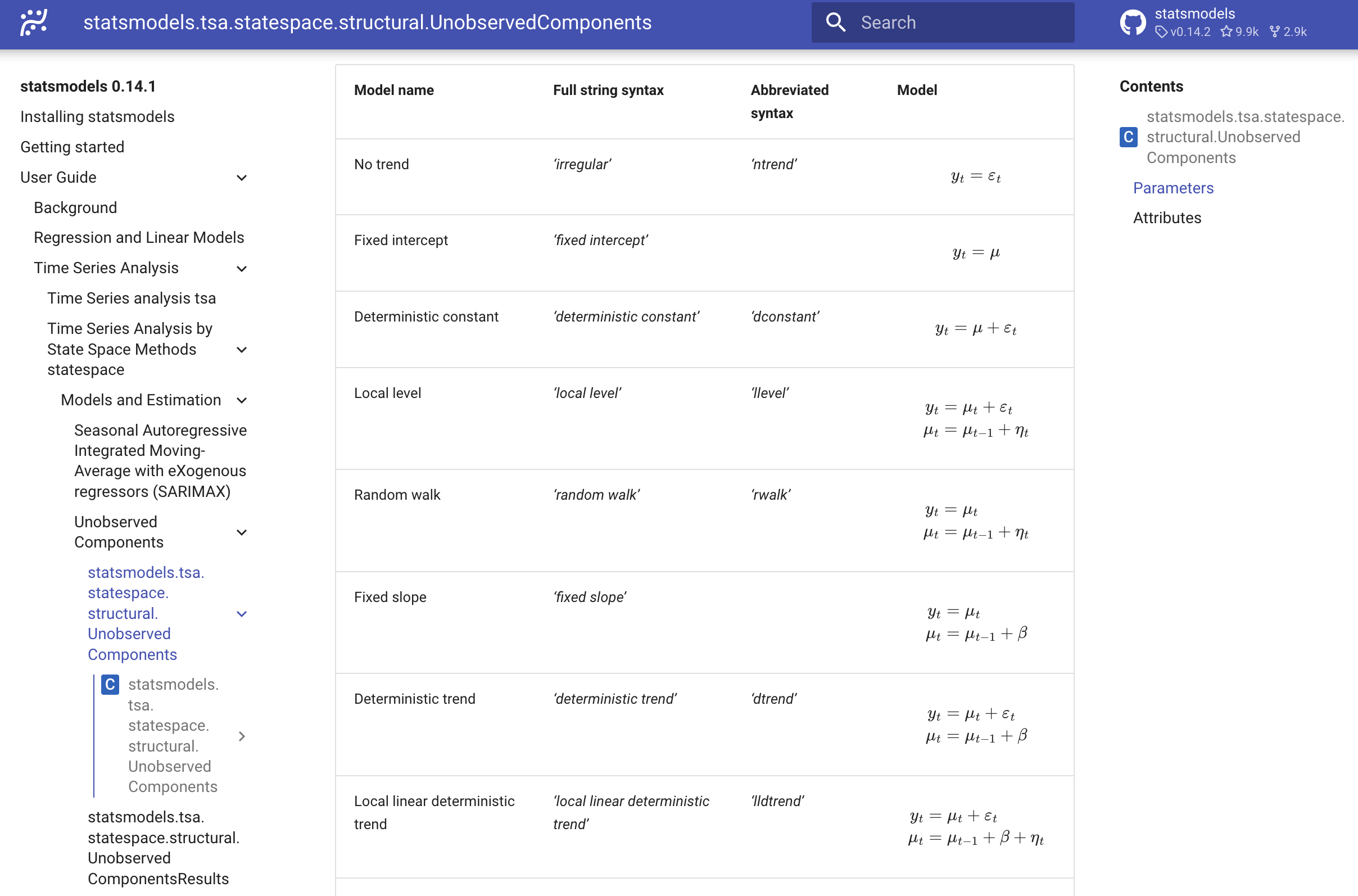
Statsmodels - Time Series Models 🤓

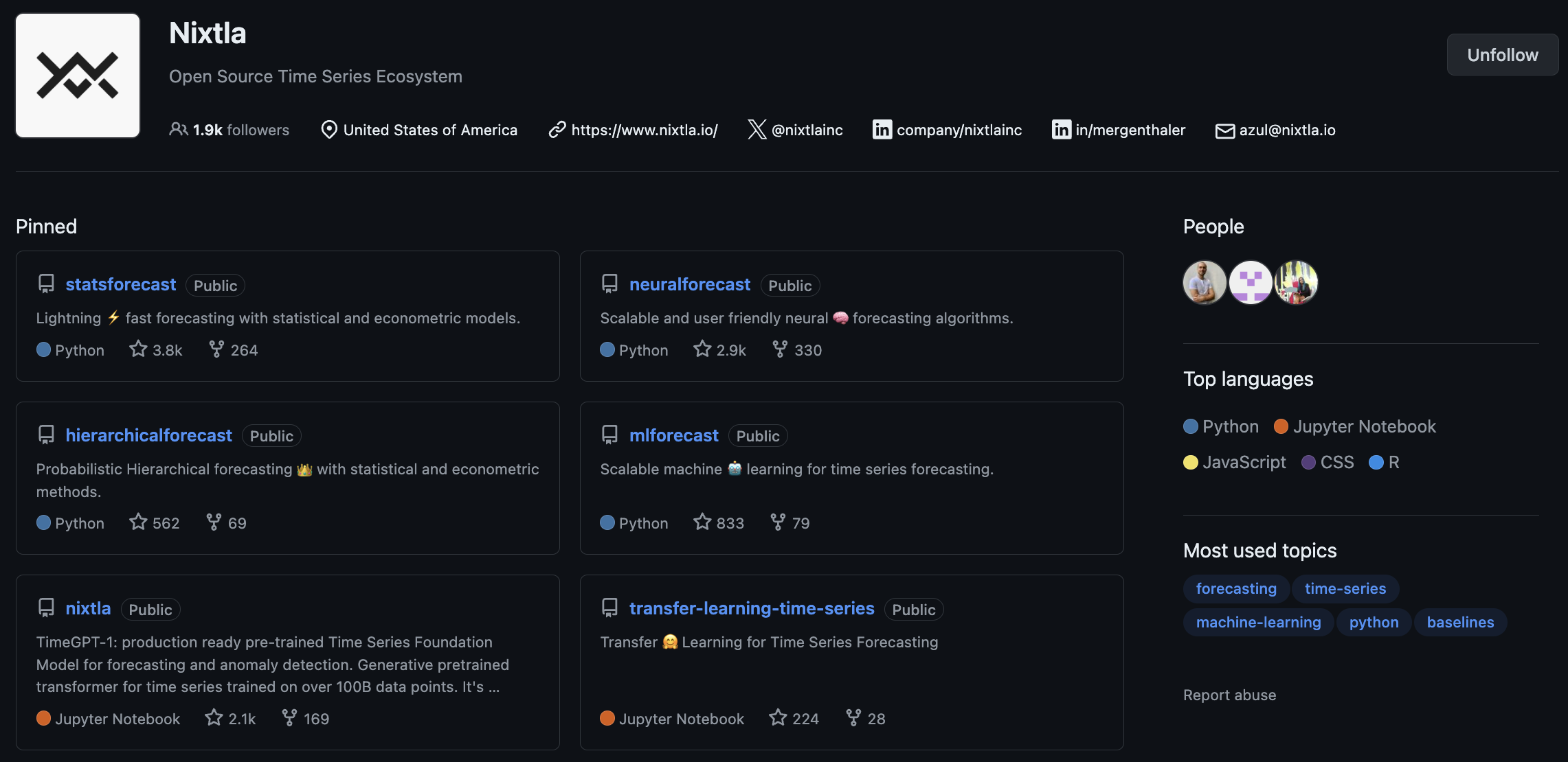
Nixtla ✨

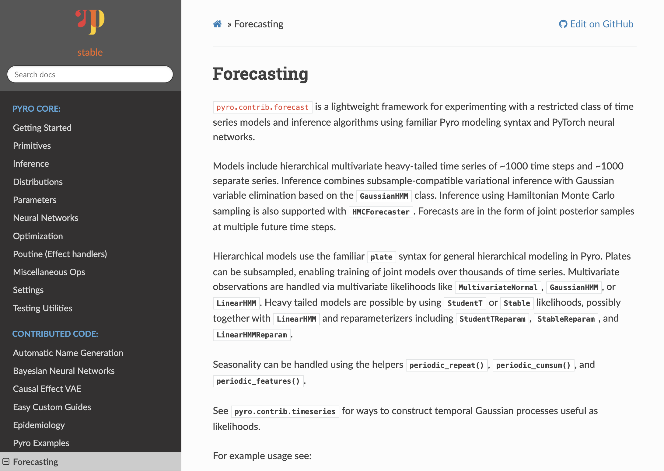
Pyro Forecasting Module 🔥

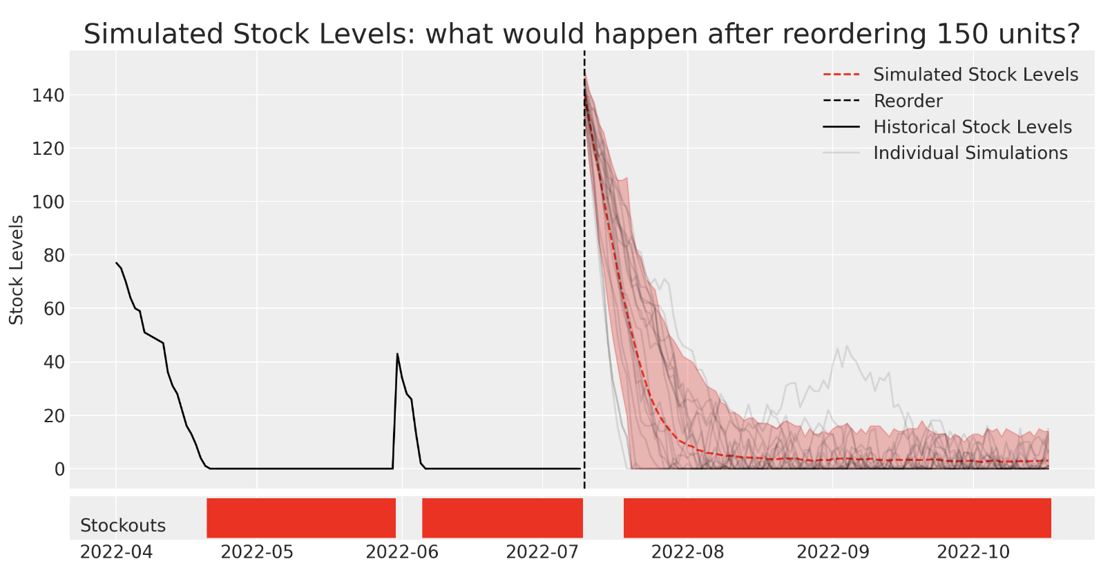
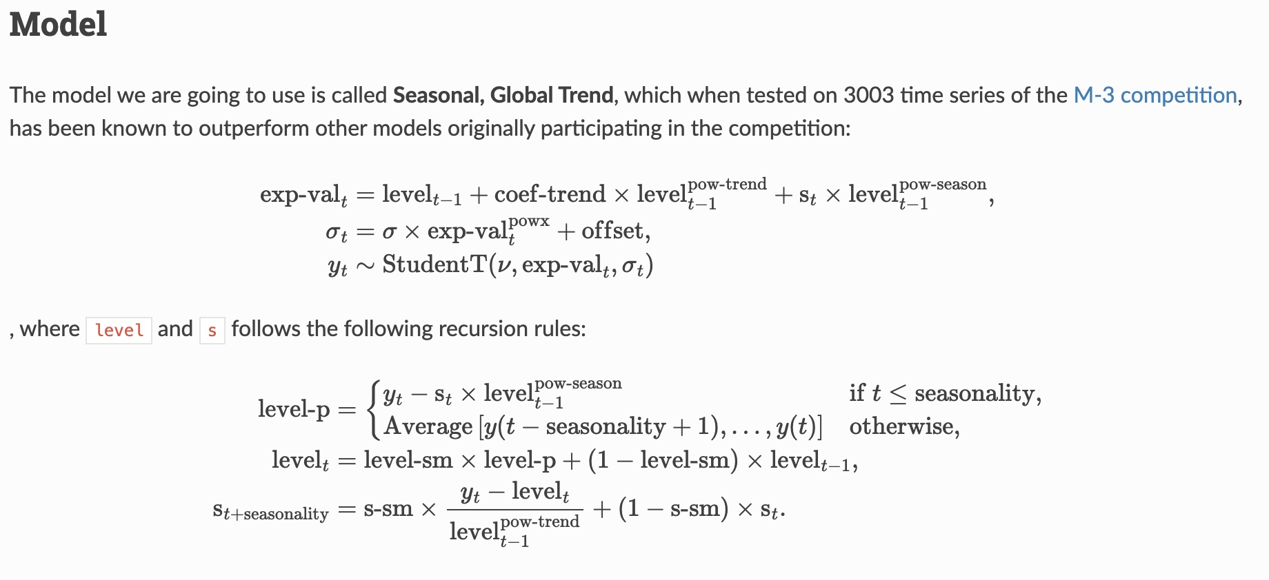
NumPyro - SGT Example Model 🫠

😅 …

Scan ⭐

An efficient implementation of for loops

def scan(f, init, xs):
  """Pure Python implementation of scan.

  Parameters
  ----------
  f : A  a Python function to be scanned.
  init : An initial loop carry value
  xs : The value over which to scan along the leading axis.
  """
  carry = init
  ys = []
  for x in xs:
    carry, y = f(carry, x)
    ys.append(y)
  return carry, np.stack(ys)

• For loop

def sum_of_powers_for_loop(phi: float, h: int) -> float:
    "phi -> 1 + phi + phi^2 + ... + phi^h"
    return sum(phi**i for i in range(1, h + 1))


assert sum_of_powers_for_loop(2, 0) == 0
assert sum_of_powers_for_loop(2, 1) == 2
assert sum_of_powers_for_loop(2, 2) == 2 + 2**2
assert sum_of_powers_for_loop(2, 3) == 2 + 2**2 + 2**3

• Scan 😎

def sum_of_powers_scan(phi, h):
    def transition_fn(carry, phi):
        power_sum, power = carry
        power = power * phi
        power_sum = power_sum + power
        return (power_sum, power), power_sum

    (power_sum, _), _ = scan(f=transition_fn, init=(0, 1), xs=jnp.ones(h) * phi)
    return power_sum

Example: Exponential Smoothing

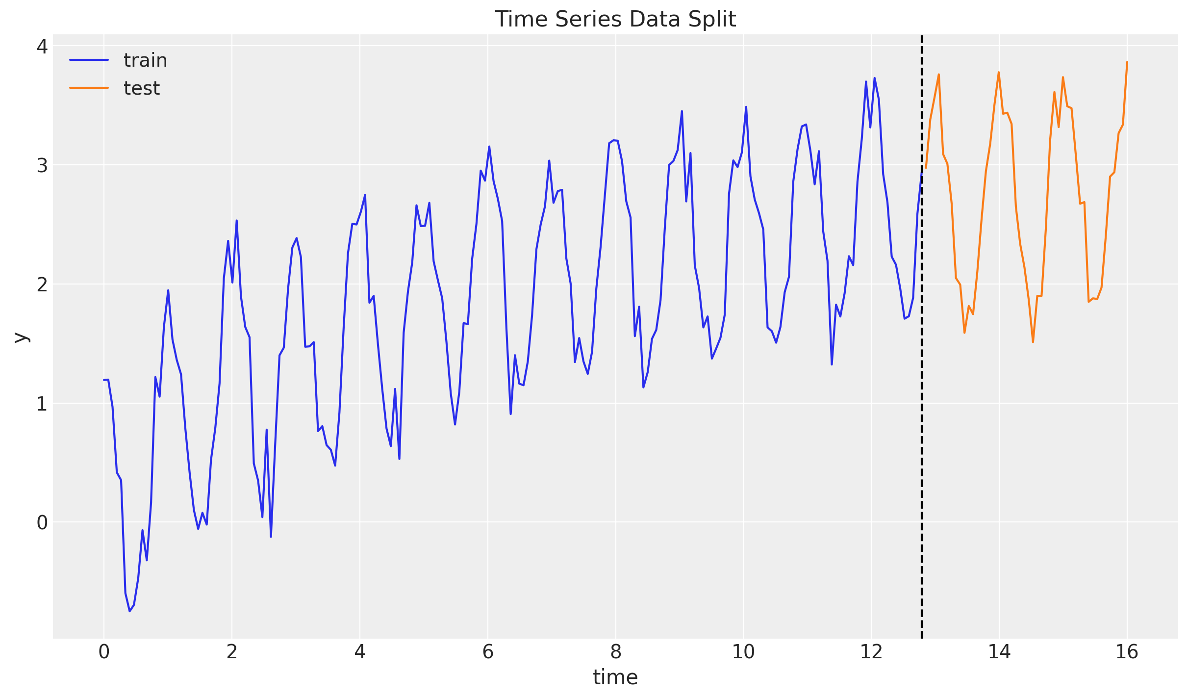
Example: Exponential Smoothing

\[ \begin{align*} \hat{y}_{t+h|t} = & \: l_t \\ l_t = & \: \alpha y_t + (1 - \alpha)l_{t-1} \end{align*} \]

• \(y_t\) is the observed value at time \(t\).
• \(\hat{y}_{t+h|t}\) is the forecast of the value at time \(t+h\) given the information up to time \(t\).
• \(l_t\) is the level at time \(t\).
• \(\alpha\) is the smoothing parameter. It is a value between 0 and 1.

Example: Exponential Smoothing

\[ \begin{align*} \hat{y}_{t+h|t} = & \: l_t \\ l_t = & \: \alpha y_t + (1 - \alpha)l_{t-1} \end{align*} \]

    def transition_fn(carry, t):
        previous_level = carry

        level = jnp.where(
            t < t_max,
            level_smoothing * y[t] + (1 - level_smoothing) * previous_level,
            previous_level,
        )

        mu = previous_level
        pred = numpyro.sample("pred", dist.Normal(loc=mu, scale=noise))

        return level, pred

Example: Exponential Smoothing

def level_model(y: ArrayLike, future: int = 0) -> None:
    # Get time series length
    t_max = y.shape[0]
    
    # --- Priors ---
    ## Level
    level_smoothing = numpyro.sample(
        "level_smoothing", dist.Beta(concentration1=1, concentration0=1)
    )
    level_init = numpyro.sample("level_init", dist.Normal(loc=0, scale=1))

    ## Noise
    noise = numpyro.sample("noise", dist.HalfNormal(scale=1))

    # --- Transition Function ---
    def transition_fn(carry, t):
        . . .

    # --- Run Scan ---
    with numpyro.handlers.condition(data={"pred": y}):
        _, preds = scan(
            transition_fn,
            level_init,
            jnp.arange(t_max + future),
        )

    # --- Forecast ---
    if future > 0:
        numpyro.deterministic("y_forecast", preds[-future:])

Example: Exponential Smoothing

Posterior Distribution Parameters

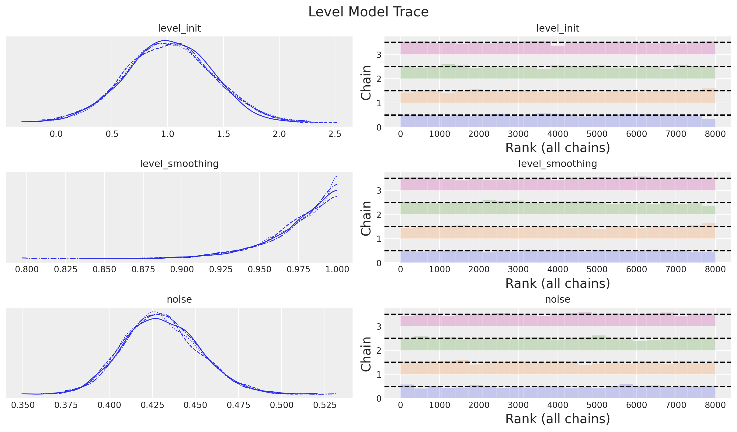
Example: Exponential Smoothing

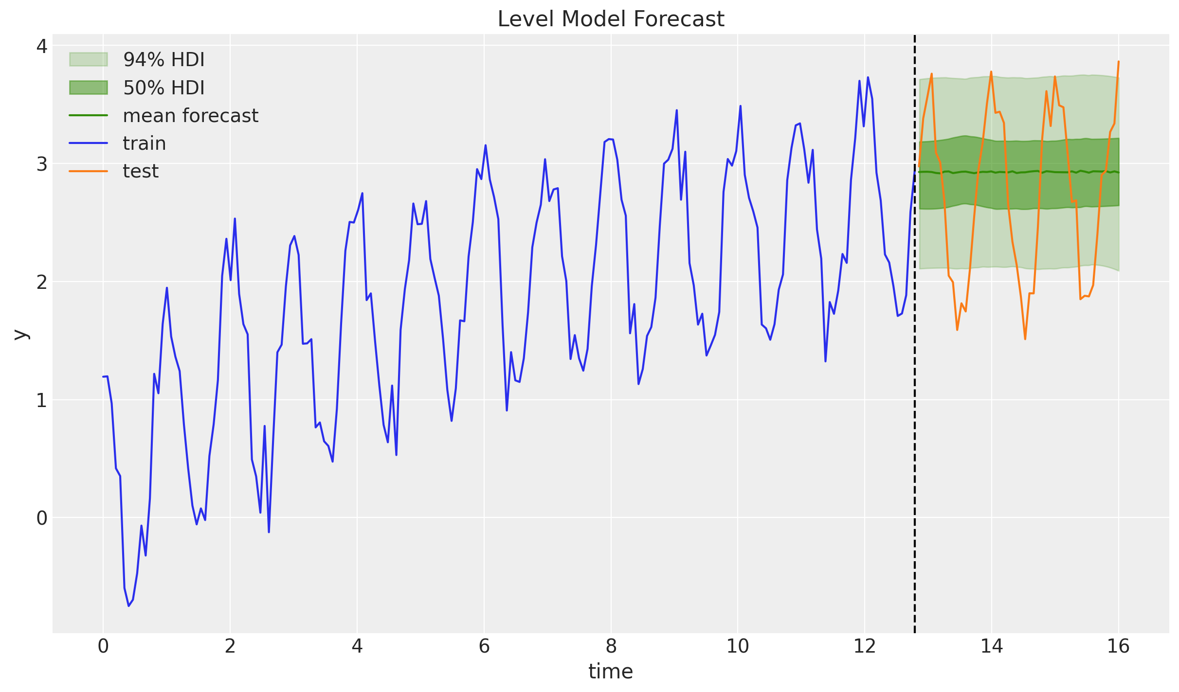
Example: Exponential Smoothing

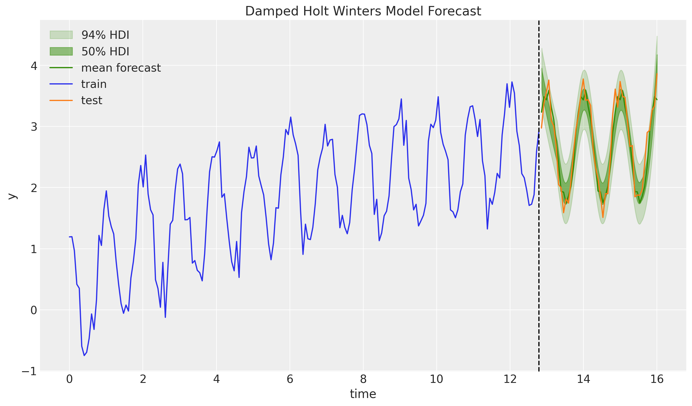
Trend + Seasonal + Damped

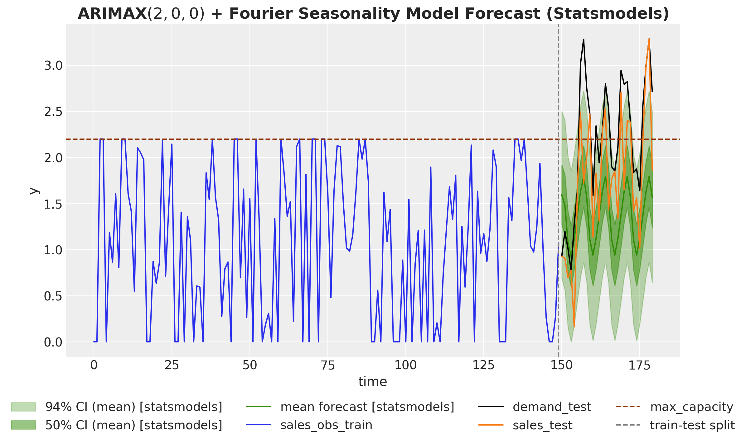
Example: ARMA(1, 1) Model

    def transition_fn(carry, t):
        y_prev, error_prev = carry
        ar_part = phi * y_prev
        ma_part = theta * error_prev
        pred = mu + ar_part + ma_part
        error = y[t] - pred
        return (y[t], error), error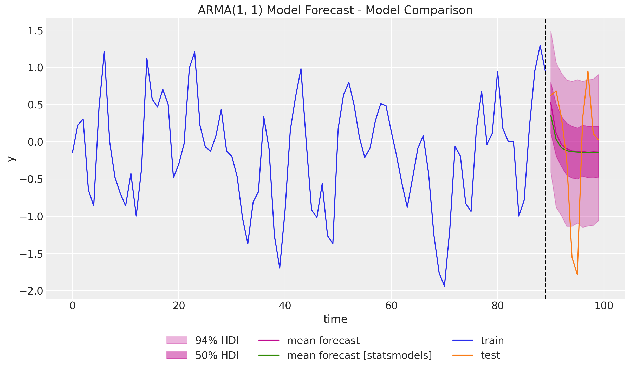

Intermittent Time Series

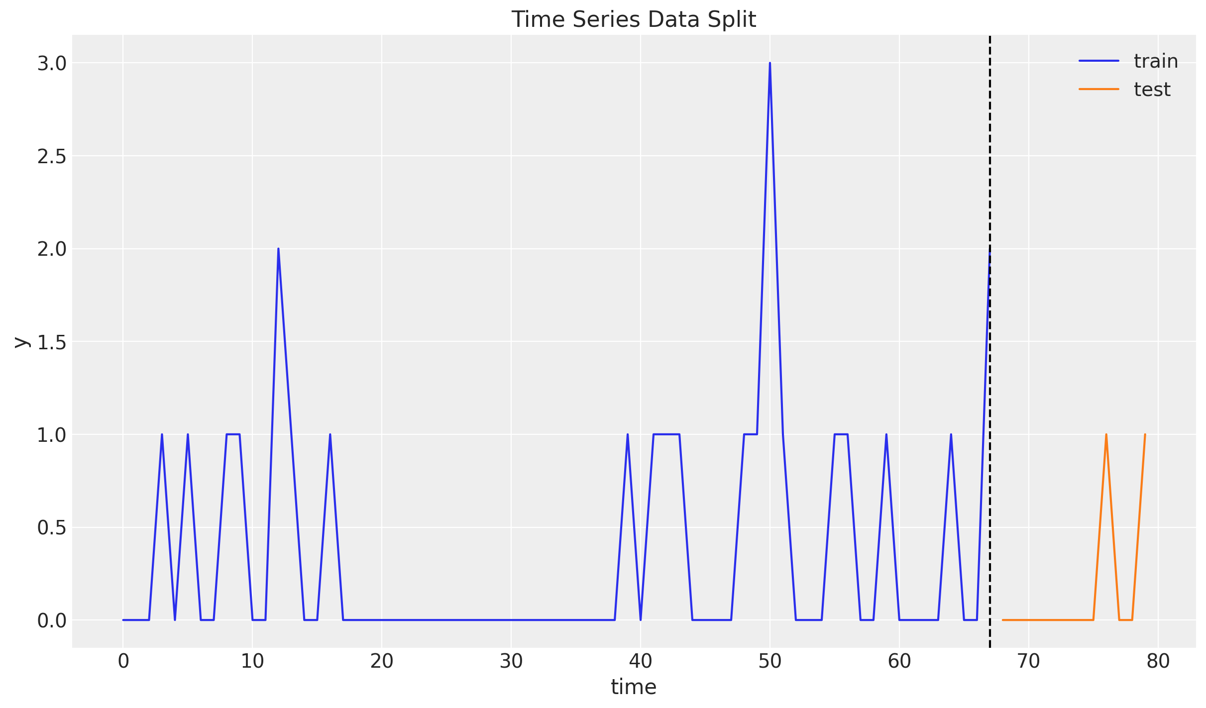
Croston’s Method

The method is based on the idea of separating the demand size \(z_t\) and the demand interval \(p_t\), and then forecasting them separately using simple exponential smoothing.

• \(z_t\): keep the non-zero values of \(y_t\).
• \(p_t\): keep the time between non-zero values of \(y_t\).

\[ \hat{y}_{t+h} = \frac{\hat{z}_{t+h}}{\hat{p}_{t+h}} \]

Croston’s Method

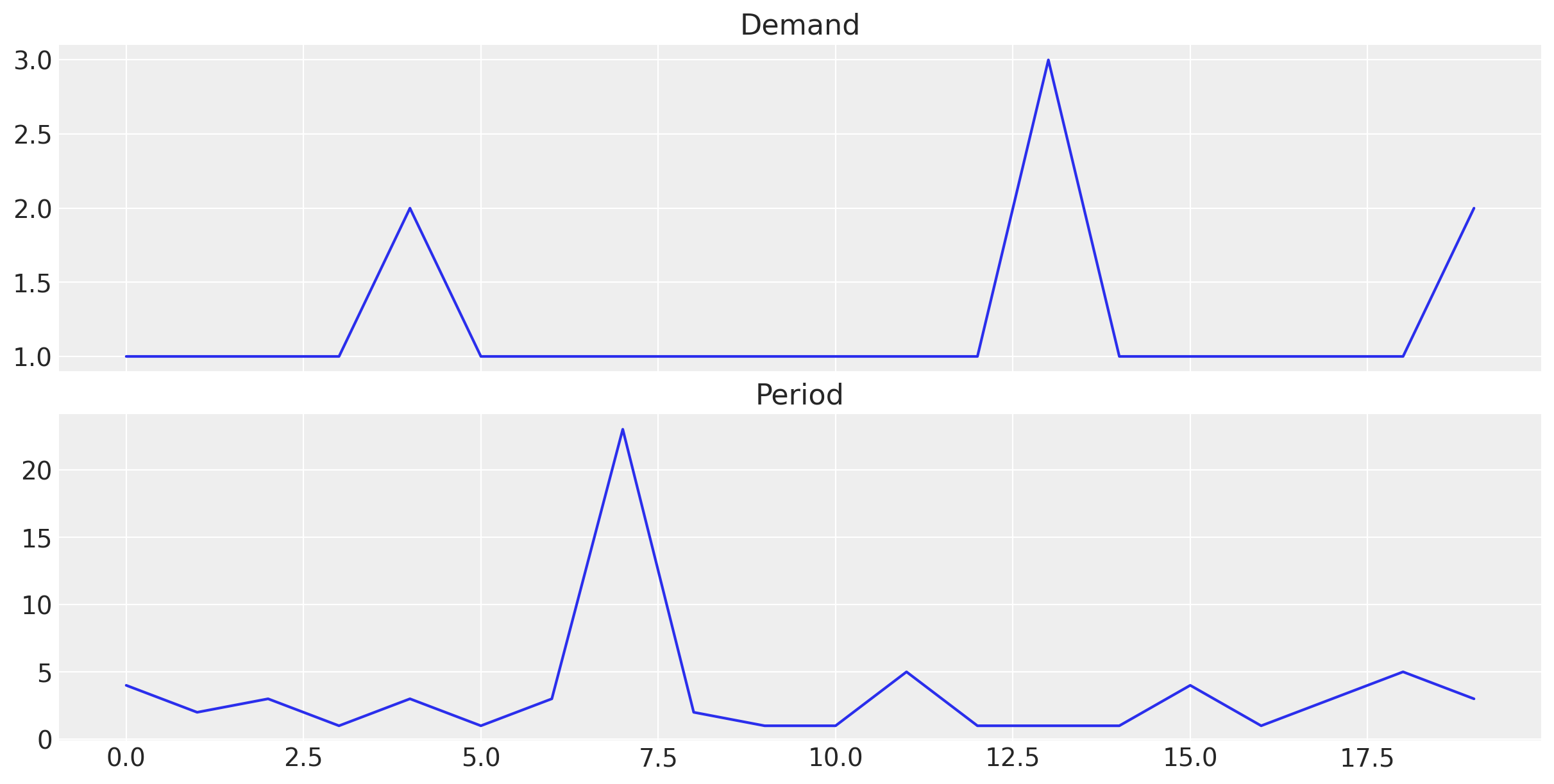
Croston’s Method

def croston_model(z: ArrayLike, p_inv: ArrayLike, future: int = 0) -> None:
    z_forecast = scope(level_model, "demand")(z, future)
    p_inv_forecast = scope(level_model, "period_inv")(p_inv, future)

    if future > 0:
        numpyro.deterministic("z_forecast", z_forecast)
        numpyro.deterministic("p_inv_forecast", p_inv_forecast)
        numpyro.deterministic("forecast", z_forecast * p_inv_forecast)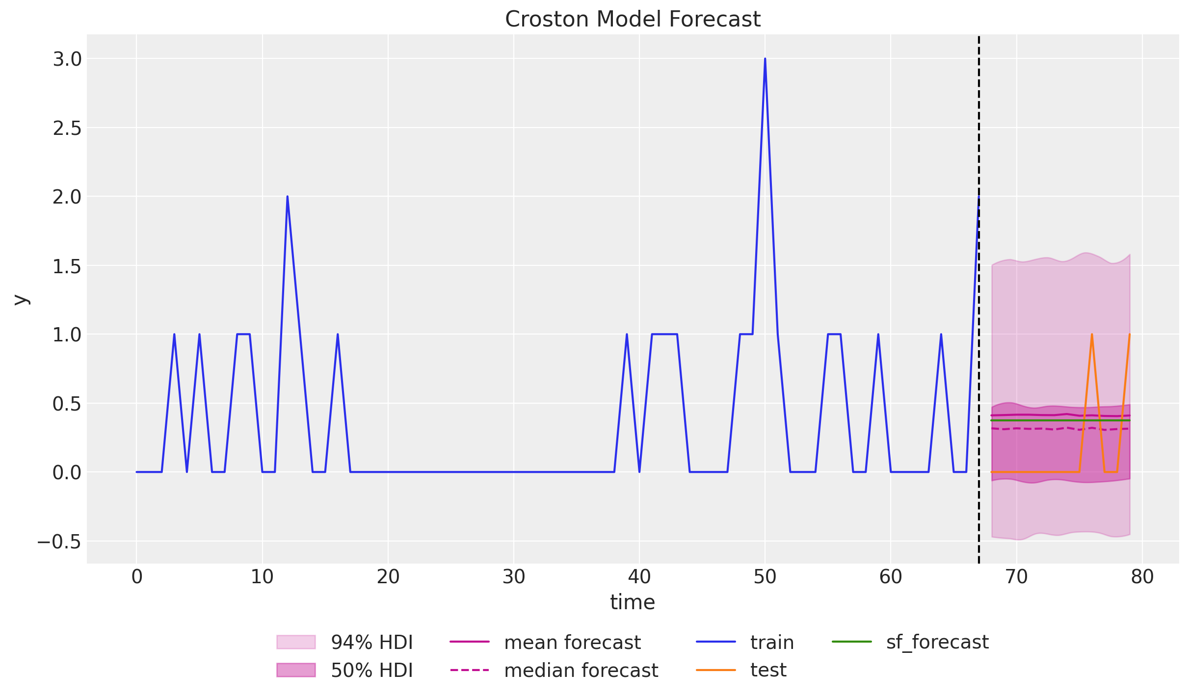

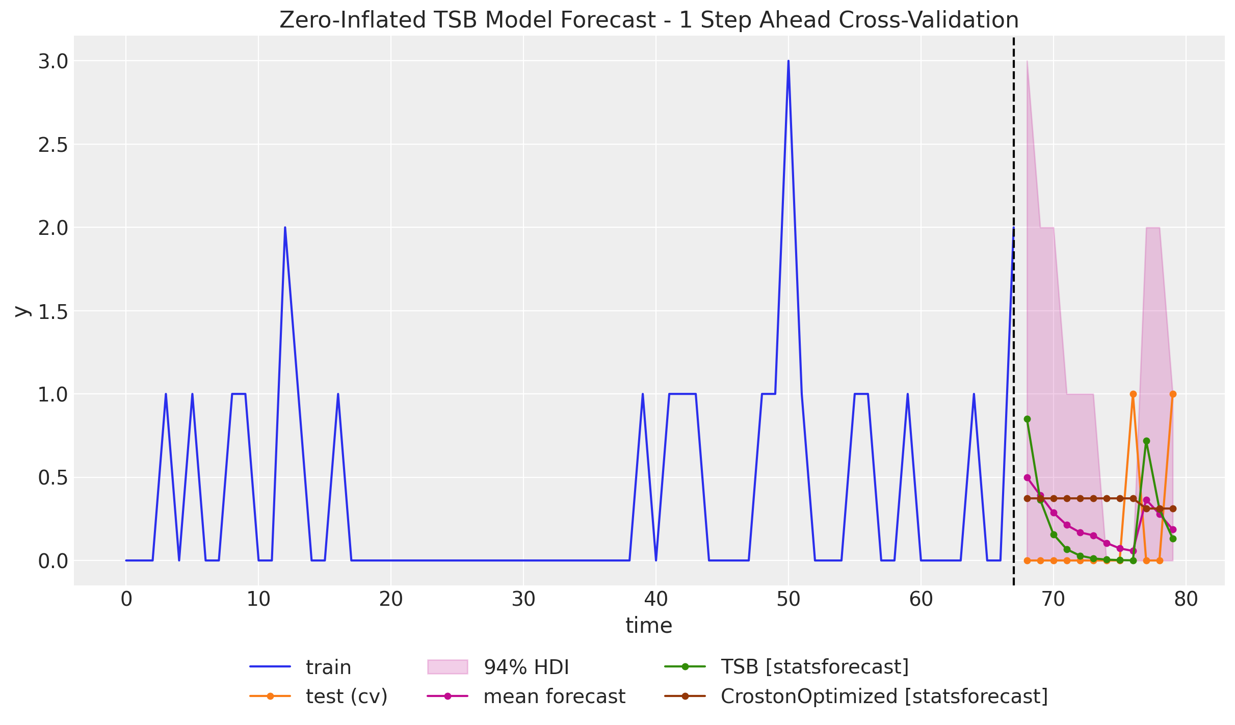
TSB Method

- The TSB method is similar to the Croston’s method: constructs two different time series out of the original one and then forecast each of them separately, so that the final forecast is generated by combining the forecasts of the two time series.

- The main difference between the two methods is that the TSB method uses the demand probability instead of the demand periods.

Zero-Inflated TSB Model

🧪 We can modify the TSB model to include zero-inflation by using a Zero-Inflated Negative Binomial Distribution.

    def transition_fn(carry, t):
        z_prev, p_prev = carry
        
        z_next . . .
        p_next . . .

        mu = z_next
        gate = 1 - p_next
        pred = numpyro.sample(
            "pred",
            dist.ZeroInflatedNegativeBinomial2(
                mean=mu, concentration=concentration, gate=gate
            ),
        )

Time-Slice Cross Validation

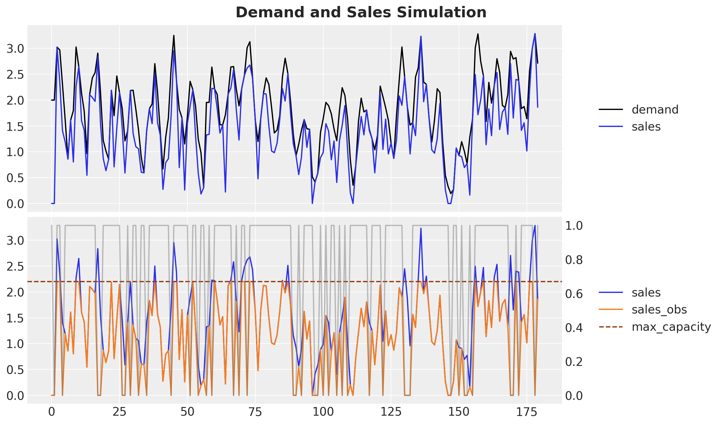
Forecasting Unseen Demand

ARIMA Model

Censored Distributions

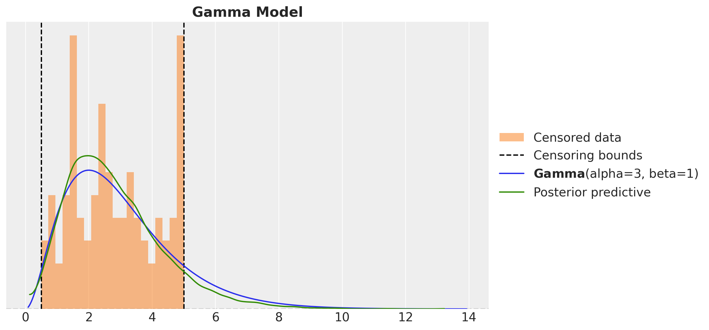
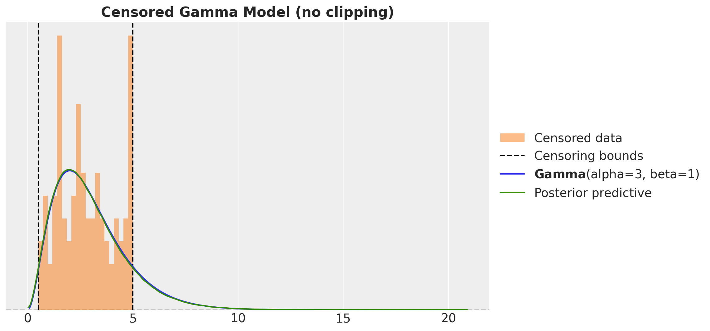
Censored Likelihood

def censored_normal(loc, scale, y, censored):
    distribution = dist.Normal(loc=loc, scale=scale)
    ccdf = 1 - distribution.cdf(y)
    numpyro.sample(
        "censored_label",
        dist.Bernoulli(probs=ccdf).mask(censored == 1),
        obs=censored
    )
    return numpyro.sample("pred", distribution.mask(censored != 1))

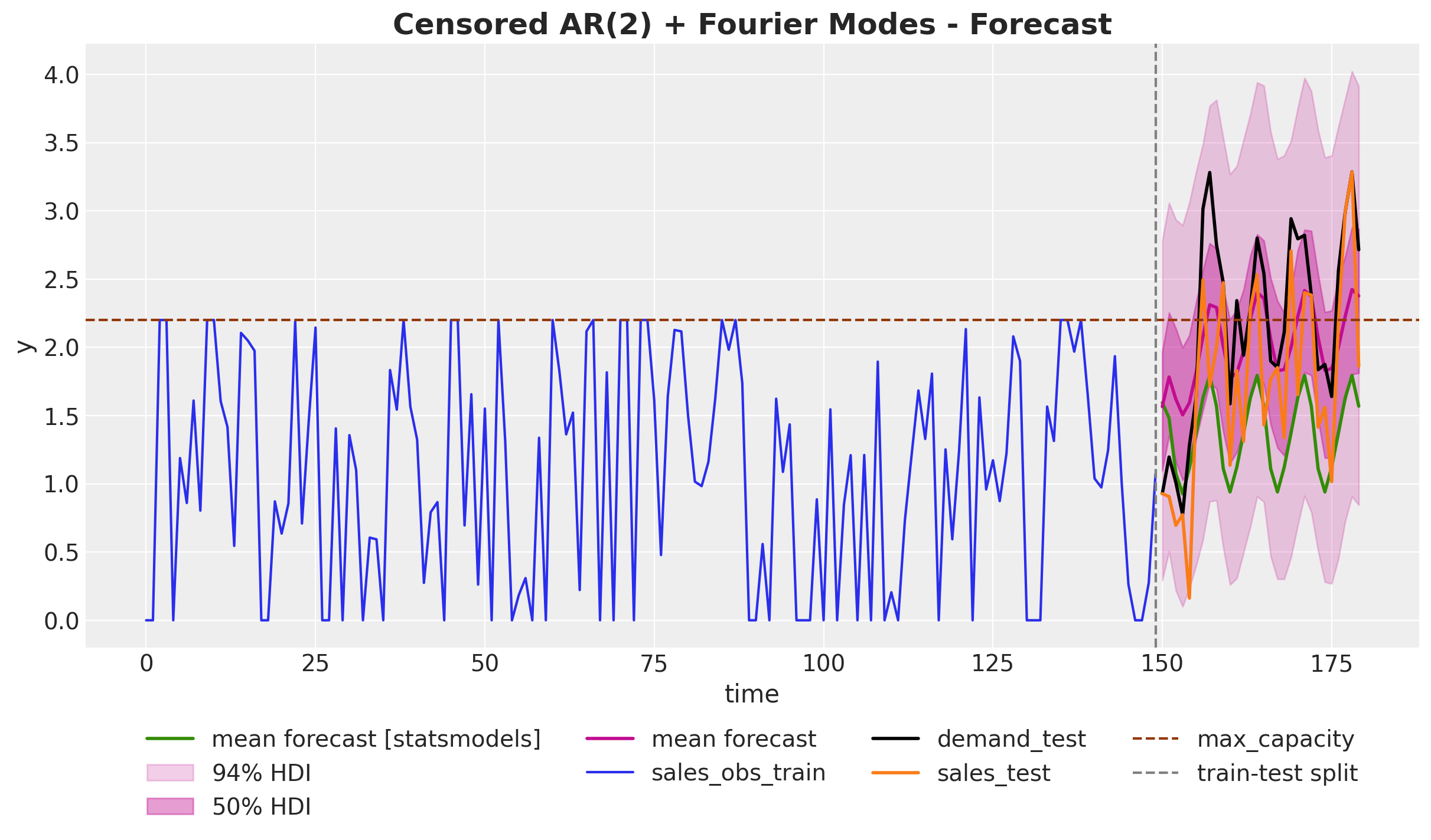
Change likelihood distribution in a time-series model:

    ## Transition function for AR(2)
    def transition_fn(carry, t):
        y_prev_1, y_prev_2 = carry
        ar_part = phi_1 * y_prev_1 + phi_2 * y_prev_2
        pred_mean = mu + ar_part + seasonal[t]
        # Censored likelihood
        pred = censored_normal(pred_mean, sigma, y[t], censored[t])
        return (pred, y_prev_1), pred

Censored Time Series Forecast 💡

Hierarchical Exponential Smoothing

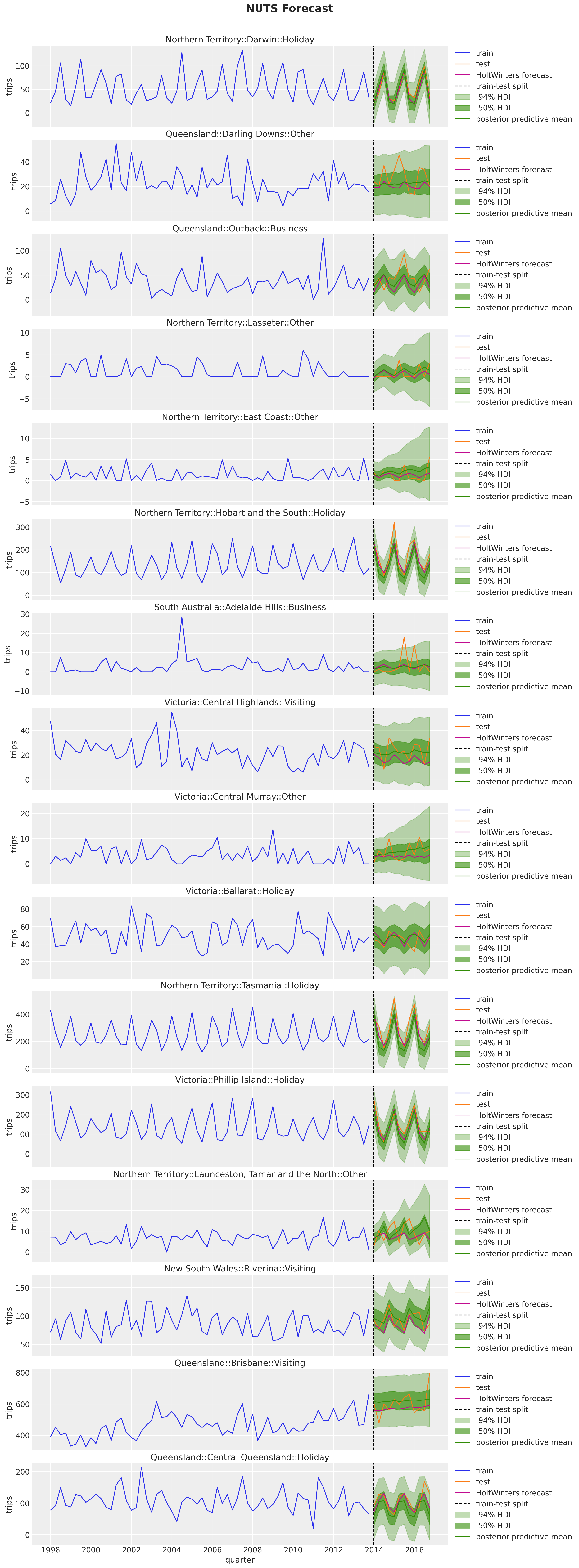
Hierarchical Exponential Smoothing

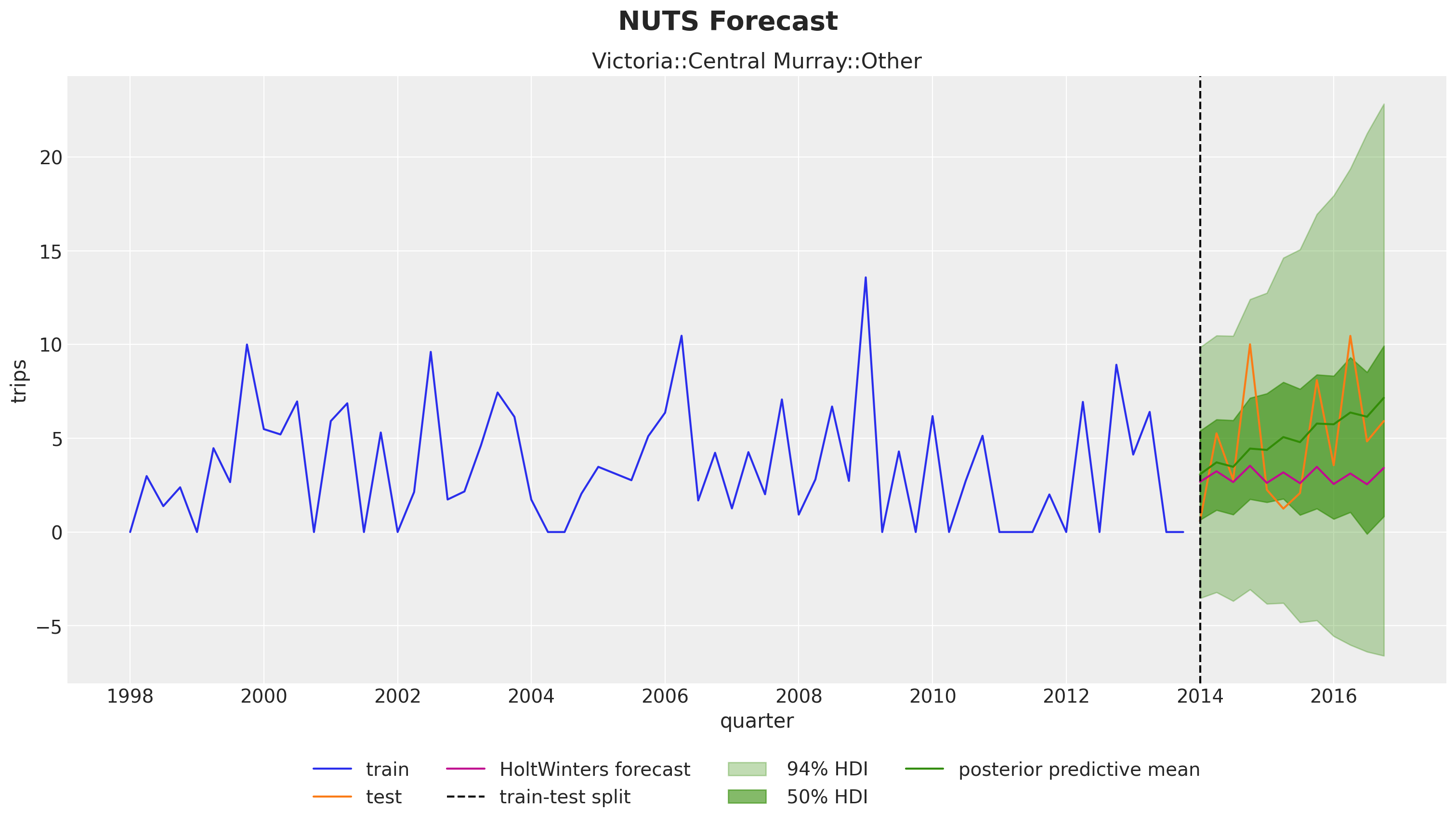
Hierarchical Exponential Smoothing

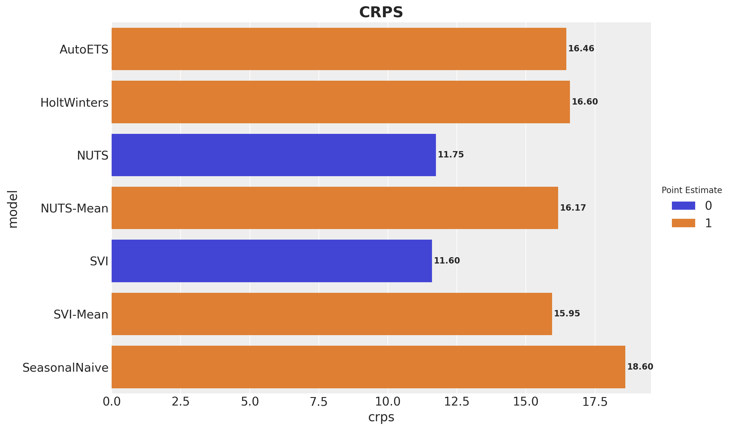
Hierarchical Pricing Elasticity Models

Idea 🤓

Use a hierarchical structure to regularize the demand elasticity parameters.

Hierarchical Pricing Elasticity Models

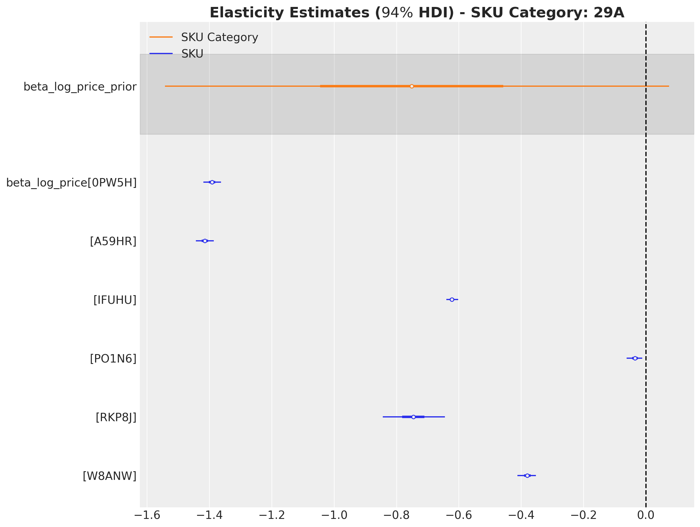
PyMC & Time Series 🚀

PyMC & Time Series 🚀

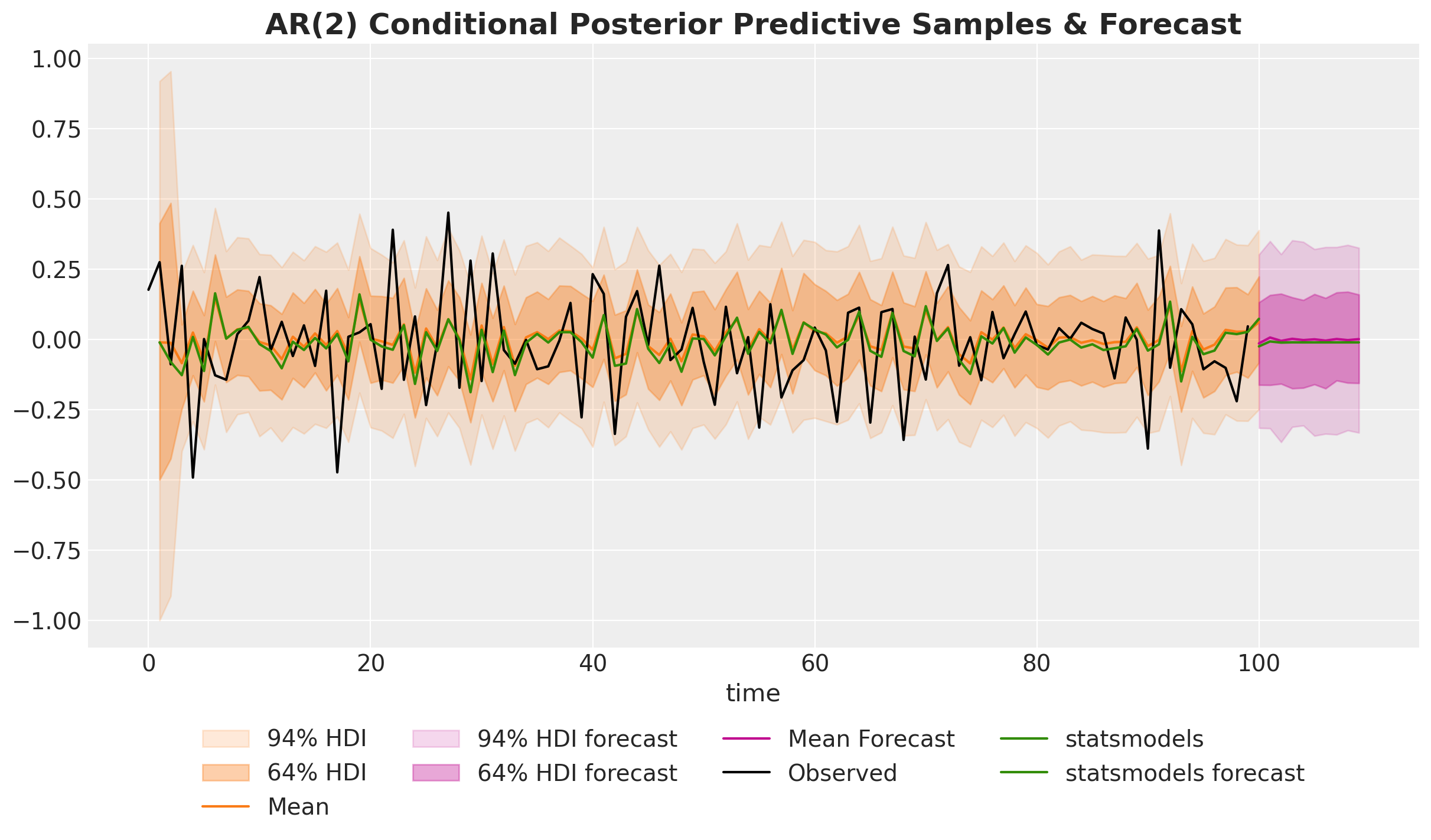
PyMC State Space Module

from pymc_experimental.statespace import structural as st

slow_trend = st.LevelTrendComponent(order=2, innovations_order=[0, 1])
seasonality = st.FrequencySeasonality(name="annual_seasonality", season_length=52, n=2, innovations=False)
exog = st.RegressionComponent(name="exog", state_names=X.columns.tolist(), innovations=False)
measurement_error = st.MeasurementError("measurement_error")

ss_mod = (slow_trend + seasonality + exog + measurement_error).build()

References

NumPyro Examples

• Notes on Exponential Smoothing with NumPyro
• Croston’s Method for Intermittent Time Series Forecasting in NumPyro
• Bayesian Censoring Data Modeling
• Demand Forecasting with Censored Likelihood
• Hierarchical Exponential Smoothing Model

PyMC Examples

• PyMC Example: Time Series Models Derived From a Generative Graph
• Time Series Analysis with Bayesian State Space Models in PyMC

Other Blogposts

• Finally! Bayesian Hierarchical Modelling at Scale
• Modeling Anything With First Principles: Demand under extreme stockouts

References

Packages:

• Nixtla
• Prophetverse
• Pyro - Forecasting
• Statsmodels - Time Series Models
• TimeSeers

Papers

• A new taxonomy for vector exponential smoothing and its application to seasonal time series

• Demand forecasting under lost sales stock policies

Thank you!

juanitorduz.github.io