We present an example of a dynamic forecasting time-series model that incorporates a prior calibration process to estimate the temperature effect on electricity demand. The model is based on the previous example Electricity Demand Forecast: Dynamic Time-Series Model. In this second iteration, we borrow the ideas from the Pyro great example Forecasting with Dynamic Linear Model (DLM) where they use a prior calibration process on a local level forecasting model. In our case, we use the same technique with a Hilbert Space Gaussian Process latent component model.
We encourage the reader to check the previous example to have a better understanding of the model. Here we focus on the calibration procedure.
Prepare Notebook
import arviz as az
import jax
import jax.numpy as jnp
import matplotlib.dates as mdates
import matplotlib.pyplot as plt
import numpy as np
import numpyro
import numpyro.distributions as dist
from jax import random
from jaxtyping import Array, Float, Int
from numpyro.contrib.hsgp.approximation import hsgp_matern
from numpyro.infer import SVI, Predictive, Trace_ELBO
from numpyro.infer.autoguide import AutoNormal

az.style.use("arviz-darkgrid")
plt.rcParams["figure.figsize"] = [12, 7]
plt.rcParams["figure.dpi"] = 100
plt.rcParams["figure.facecolor"] = "white"

numpyro.set_host_device_count(n=4)

rng_key = random.PRNGKey(seed=42)

%load_ext autoreload
%autoreload 2
%load_ext jaxtyping
%jaxtyping.typechecker beartype.beartype
%config InlineBackend.figure_format = "retina"
Load Data
We load the data as in the previous example.
demand_dates = np.arange("2014-01-01", "2014-02-26", dtype="datetime64[h]")
demand_loc = mdates.WeekdayLocator(byweekday=mdates.WE)
demand_fmt = mdates.DateFormatter("%a %b %d")

demand = jnp.array(
    np.array(
        "3.794,3.418,3.152,3.026,3.022,3.055,3.180,3.276,3.467,3.620,3.730,3.858,3.851,3.839,3.861,3.912,4.082,4.118,4.011,3.965,3.932,3.693,3.585,4.001,3.623,3.249,3.047,3.004,3.104,3.361,3.749,3.910,4.075,4.165,4.202,4.225,4.265,4.301,4.381,4.484,4.552,4.440,4.233,4.145,4.116,3.831,3.712,4.121,3.764,3.394,3.159,3.081,3.216,3.468,3.838,4.012,4.183,4.269,4.280,4.310,4.315,4.233,4.188,4.263,4.370,4.308,4.182,4.075,4.057,3.791,3.667,4.036,3.636,3.283,3.073,3.003,3.023,3.113,3.335,3.484,3.697,3.723,3.786,3.763,3.748,3.714,3.737,3.828,3.937,3.929,3.877,3.829,3.950,3.756,3.638,4.045,3.682,3.283,3.036,2.933,2.956,2.959,3.157,3.236,3.370,3.493,3.516,3.555,3.570,3.656,3.792,3.950,3.953,3.926,3.849,3.813,3.891,3.683,3.562,3.936,3.602,3.271,3.085,3.041,3.201,3.570,4.123,4.307,4.481,4.533,4.545,4.524,4.470,4.457,4.418,4.453,4.539,4.473,4.301,4.260,4.276,3.958,3.796,4.180,3.843,3.465,3.246,3.203,3.360,3.808,4.328,4.509,4.598,4.562,4.566,4.532,4.477,4.442,4.424,4.486,4.579,4.466,4.338,4.270,4.296,4.034,3.877,4.246,3.883,3.520,3.306,3.252,3.387,3.784,4.335,4.465,4.529,4.536,4.589,4.660,4.691,4.747,4.819,4.950,4.994,4.798,4.540,4.352,4.370,4.047,3.870,4.245,3.848,3.509,3.302,3.258,3.419,3.809,4.363,4.605,4.793,4.908,5.040,5.204,5.358,5.538,5.708,5.888,5.966,5.817,5.571,5.321,5.141,4.686,4.367,4.618,4.158,3.771,3.555,3.497,3.646,4.053,4.687,5.052,5.342,5.586,5.808,6.038,6.296,6.548,6.787,6.982,7.035,6.855,6.561,6.181,5.899,5.304,4.795,4.862,4.264,3.820,3.588,3.481,3.514,3.632,3.857,4.116,4.375,4.462,4.460,4.422,4.398,4.407,4.480,4.621,4.732,4.735,4.572,4.385,4.323,4.069,3.940,4.247,3.821,3.416,3.220,3.124,3.132,3.181,3.337,3.469,3.668,3.788,3.834,3.894,3.964,4.109,4.275,4.472,4.623,4.703,4.594,4.447,4.459,4.137,3.913,4.231,3.833,3.475,3.302,3.279,3.519,3.975,4.600,4.864,5.104,5.308,5.542,5.759,6.005,6.285,6.617,6.993,7.207,7.095,6.839,6.387,6.048,5.433,4.904,4.959,4.425,4.053,3.843,3.823,4.017,4.521,5.229,5.802,6.449,6.975,7.506,7.973,8.359,8.596,8.794,9.030,9.090,8.885,8.525,8.147,7.797,6.938,6.215,6.123,5.495,5.140,4.896,4.812,5.024,5.536,6.293,7.000,7.633,8.030,8.459,8.768,9.000,9.113,9.155,9.173,9.039,8.606,8.095,7.617,7.208,6.448,5.740,5.718,5.106,4.763,4.610,4.566,4.737,5.204,5.988,6.698,7.438,8.040,8.484,8.837,9.052,9.114,9.214,9.307,9.313,9.006,8.556,8.275,7.911,7.077,6.348,6.175,5.455,5.041,4.759,4.683,4.908,5.411,6.199,6.923,7.593,8.090,8.497,8.843,9.058,9.159,9.231,9.253,8.852,7.994,7.388,6.735,6.264,5.690,5.227,5.220,4.593,4.213,3.984,3.891,3.919,4.031,4.287,4.558,4.872,4.963,5.004,5.017,5.057,5.064,5.000,5.023,5.007,4.923,4.740,4.586,4.517,4.236,4.055,4.337,3.848,3.473,3.273,3.198,3.204,3.252,3.404,3.560,3.767,3.896,3.934,3.972,3.985,4.032,4.122,4.239,4.389,4.499,4.406,4.356,4.396,4.106,3.914,4.265,3.862,3.546,3.360,3.359,3.649,4.180,4.813,5.086,5.301,5.384,5.434,5.470,5.529,5.582,5.618,5.636,5.561,5.291,5.000,4.840,4.767,4.364,4.160,4.452,4.011,3.673,3.503,3.483,3.695,4.213,4.810,5.028,5.149,5.182,5.208,5.179,5.190,5.220,5.202,5.216,5.232,5.019,4.828,4.686,4.657,4.304,4.106,4.389,3.955,3.643,3.489,3.479,3.695,4.187,4.732,4.898,4.997,5.001,5.022,5.052,5.094,5.143,5.178,5.250,5.255,5.075,4.867,4.691,4.665,4.352,4.121,4.391,3.966,3.615,3.437,3.430,3.666,4.149,4.674,4.851,5.011,5.105,5.242,5.378,5.576,5.790,6.030,6.254,6.340,6.253,6.039,5.736,5.490,4.936,4.580,4.742,4.230,3.895,3.712,3.700,3.906,4.364,4.962,5.261,5.463,5.495,5.477,5.394,5.250,5.159,5.081,5.083,5.038,4.857,4.643,4.526,4.428,4.141,3.975,4.290,3.809,3.423,3.217,3.132,3.192,3.343,3.606,3.803,3.963,3.998,3.962,3.894,3.814,3.776,3.808,3.914,4.033,4.079,4.027,3.974,4.057,3.859,3.759,4.132,3.716,3.325,3.111,3.030,3.046,3.096,3.254,3.390,3.606,3.718,3.755,3.768,3.768,3.834,3.957,4.199,4.393,4.532,4.516,4.380,4.390,4.142,3.954,4.233,3.795,3.425,3.209,3.124,3.177,3.288,3.498,3.715,4.092,4.383,4.644,4.909,5.184,5.518,5.889,6.288,6.643,6.729,6.567,6.179,5.903,5.278,4.788,4.885,4.363,4.011,3.823,3.762,3.998,4.598,5.349,5.898,6.487,6.941,7.381,7.796,8.185,8.522,8.825,9.103,9.198,8.889,8.174,7.214,6.481,5.611,5.026,5.052,4.484,4.148,3.955,3.873,4.060,4.626,5.272,5.441,5.535,5.534,5.610,5.671,5.724,5.793,5.838,5.908,5.868,5.574,5.276,5.065,4.976,4.554,4.282,4.547,4.053,3.720,3.536,3.524,3.792,4.420,5.075,5.208,5.344,5.482,5.701,5.936,6.210,6.462,6.683,6.979,7.059,6.893,6.535,6.121,5.797,5.152,4.705,4.805,4.272,3.975,3.805,3.775,3.996,4.535,5.275,5.509,5.730,5.870,6.034,6.175,6.340,6.500,6.603,6.804,6.787,6.460,6.043,5.627,5.367,4.866,4.575,4.728,4.157,3.795,3.607,3.537,3.596,3.803,4.125,4.398,4.660,4.853,5.115,5.412,5.669,5.930,6.216,6.466,6.641,6.605,6.316,5.821,5.520,5.016,4.657,4.746,4.197,3.823,3.613,3.505,3.488,3.532,3.716,4.011,4.421,4.836,5.296,5.766,6.233,6.646,7.011,7.380,7.660,7.804,7.691,7.364,7.019,6.260,5.545,5.437,4.806,4.457,4.235,4.172,4.396,5.002,5.817,6.266,6.732,7.049,7.184,7.085,6.798,6.632,6.408,6.218,5.968,5.544,5.217,4.964,4.758,4.328,4.074,4.367,3.883,3.536,3.404,3.396,3.624,4.271,4.916,4.953,5.016,5.048,5.106,5.124,5.200,5.244,5.242,5.341,5.368,5.166,4.910,4.762,4.700,4.276,4.035,4.318,3.858,3.550,3.399,3.382,3.590,4.261,4.937,4.994,5.094,5.168,5.303,5.410,5.571,5.740,5.900,6.177,6.274,6.039,5.700,5.389,5.192,4.672,4.359,4.614,4.118,3.805,3.627,3.646,3.882,4.470,5.106,5.274,5.507,5.711,5.950,6.200,6.527,6.884,7.196,7.615,7.845,7.759,7.437,7.059,6.584,5.742,5.125,5.139,4.564,4.218,4.025,4.000,4.245,4.783,5.504,5.920,6.271,6.549,6.894,7.231,7.535,7.597,7.562,7.609,7.534,7.118,6.448,5.963,5.565,5.005,4.666,4.850,4.302,3.905,3.678,3.610,3.672,3.869,4.204,4.541,4.944,5.265,5.651,6.090,6.547,6.935,7.318,7.625,7.793,7.760,7.510,7.145,6.805,6.103,5.520,5.462,4.824,4.444,4.237,4.157,4.164,4.275,4.545,5.033,5.594,6.176,6.681,6.628,6.238,6.039,5.897,5.832,5.701,5.483,4.949,4.589,4.407,4.027,3.820,4.075,3.650,3.388,3.271,3.268,3.498,4.086,4.800,4.933,5.102,5.126,5.194,5.260,5.319,5.364,5.419,5.559,5.568,5.332,5.027,4.864,4.738,4.303,4.093,4.379,3.952,3.632,3.461,3.446,3.732,4.294,4.911,5.021,5.138,5.223,5.348,5.479,5.661,5.832,5.966,6.178,6.212,5.949,5.640,5.449,5.213,4.678,4.376,4.601,4.147,3.815,3.610,3.605,3.879,4.468,5.090,5.226,5.406,5.561,5.740,5.899,6.095,6.272,6.402,6.610,6.585,6.265,5.925,5.747,5.497,4.932,4.580,4.763,4.298,4.026,3.871,3.827,4.065,4.643,5.317,5.494,5.685,5.814,5.912,5.999,6.097,6.176,6.136,6.131,6.049,5.796,5.532,5.475,5.254,4.742,4.453,4.660,4.176,3.895,3.726,3.717,3.910,4.479,5.135,5.306,5.520,5.672,5.737,5.785,5.829,5.893,5.892,5.921,5.817,5.557,5.304,5.234,5.074,4.656,4.396,4.599,4.064,3.749,3.560,3.475,3.552,3.783,4.045,4.258,4.539,4.762,4.938,5.049,5.037,5.066,5.151,5.197,5.201,5.132,4.908,4.725,4.568,4.222,3.939,4.215,3.741,3.380,3.174,3.076,3.071,3.172,3.328,3.427,3.603,3.738,3.765,3.777,3.705,3.690,3.742,3.859,4.032,4.113,4.032,4.066,4.011,3.712,3.530,3.905,3.556,3.283,3.136,3.146,3.400,4.009,4.717,4.827,4.909,4.973,5.036,5.079,5.160,5.228,5.241,5.343,5.350,5.184,4.941,4.797,4.615,4.160,3.904,4.213,3.810,3.528,3.369,3.381,3.609,4.178,4.861,4.918,5.006,5.102,5.239,5.385,5.528,5.724,5.845,6.048,6.097,5.838,5.507,5.267,5.003,4.462,4.184,4.431,3.969,3.660,3.480,3.470,3.693,4.313,4.955,5.083,5.251,5.268,5.293,5.285,5.308,5.349,5.322,5.328,5.151,4.975,4.741,4.678,4.458,4.056,3.868,4.226,3.799,3.428,3.253,3.228,3.452,4.040,4.726,4.709,4.721,4.741,4.846,4.864,4.868,4.836,4.799,4.890,4.946,4.800,4.646,4.693,4.546,4.117,3.897,4.259,3.893,3.505,3.341,3.334,3.623,4.240,4.925,4.986,5.028,4.987,4.984,4.975,4.912,4.833,4.686,4.710,4.718,4.577,4.454,4.532,4.407,4.064,3.883,4.221,3.792,3.445,3.261,3.221,3.295,3.521,3.804,4.038,4.200,4.226,4.198,4.182,4.078,4.018,4.002,4.066,4.158,4.154,4.084,4.104,4.001,3.773,3.700,4.078,3.702,3.349,3.143,3.052,3.070,3.181,3.327,3.440,3.616,3.678,3.694,3.710,3.706,3.764,3.852,4.009,4.202,4.323,4.249,4.275,4.162,3.848,3.706,4.060,3.703,3.401,3.251,3.239,3.455,4.041,4.743,4.815,4.916,4.931,4.966,5.063,5.218,5.381,5.458,5.550,5.566,5.376,5.104,5.022,4.793,4.335,4.108,4.410,4.008,3.666,3.497,3.464,3.698,4.333,4.998,5.094,5.272,5.459,5.648,5.853,6.062,6.258,6.236,6.226,5.957,5.455,5.066,4.968,4.742,4.304,4.105,4.410".split(
            ","
        )
    ).astype(np.float32)
)

temperature = jnp.array(
    np.array(
        "18.050,17.200,16.450,16.650,16.400,17.950,19.700,20.600,22.350,23.700,24.800,25.900,25.300,23.650,20.700,19.150,22.650,22.650,22.400,22.150,22.050,22.150,21.000,19.500,18.450,17.250,16.300,15.700,15.500,15.450,15.650,16.500,18.100,17.800,19.100,19.850,20.300,21.050,22.800,21.650,20.150,19.300,18.750,17.900,17.350,16.850,16.350,15.700,14.950,14.500,14.350,14.450,14.600,14.600,14.700,15.450,16.700,18.300,20.100,20.650,19.450,20.200,20.250,20.050,20.250,20.950,21.900,21.000,19.900,19.250,17.300,16.300,15.800,15.000,14.400,14.050,13.650,13.500,14.150,15.300,14.800,17.050,18.350,19.450,18.550,18.650,18.850,19.800,19.650,18.900,19.500,17.700,17.350,16.950,16.400,15.950,14.900,14.250,13.050,12.000,11.500,10.950,12.300,16.100,17.100,19.600,21.100,22.600,24.350,25.250,25.750,20.350,15.550,18.300,19.400,19.250,18.550,17.700,16.750,15.800,14.900,14.050,14.100,13.500,13.000,12.950,13.300,13.900,15.400,16.750,17.300,17.750,18.400,18.500,18.800,19.450,18.750,18.400,16.950,15.800,15.350,15.250,15.150,14.900,14.500,14.600,14.400,14.150,14.300,14.500,14.950,15.550,15.800,15.550,16.450,17.500,17.700,18.750,19.600,19.900,19.350,19.550,17.900,16.400,15.550,14.900,14.400,13.950,13.300,12.950,12.650,12.450,12.350,12.150,11.950,14.150,15.850,17.750,19.450,22.150,23.850,23.450,24.950,26.850,26.100,25.150,23.250,21.300,19.850,18.900,18.250,17.450,17.100,16.400,15.550,15.050,14.400,14.550,15.150,17.050,18.850,20.850,24.250,27.700,28.400,30.750,30.700,32.200,31.750,30.650,29.750,28.850,27.850,25.950,24.700,24.850,24.050,23.850,23.500,22.950,22.200,21.750,22.350,24.050,25.150,27.100,28.050,29.750,31.250,31.900,32.950,33.150,33.950,33.850,33.250,32.500,31.500,28.300,23.900,22.900,22.300,21.250,20.500,19.850,18.850,18.300,18.100,18.200,18.150,18.000,17.700,18.250,19.700,20.750,21.800,21.500,21.600,20.800,19.400,18.400,17.900,17.600,17.550,17.550,17.650,17.400,17.150,16.800,17.000,16.900,17.200,17.350,17.650,17.800,18.400,19.300,20.200,21.050,21.700,21.800,21.800,21.500,20.000,19.300,18.200,18.100,17.700,16.950,16.250,15.600,15.500,15.300,15.450,15.500,15.750,17.350,19.150,21.650,24.700,25.200,24.300,26.900,28.100,29.450,29.850,29.450,26.350,27.050,25.700,25.150,23.850,22.450,21.450,20.850,20.700,21.300,21.550,20.800,22.300,26.300,32.600,35.150,36.800,38.150,39.950,40.850,41.250,42.300,41.950,41.350,40.600,36.350,36.150,34.600,34.050,35.400,36.300,35.550,33.700,30.650,29.450,29.500,31.000,33.300,35.700,36.650,37.650,39.400,40.600,40.250,37.550,37.300,35.400,32.750,31.200,29.600,28.350,27.500,28.750,28.900,29.900,28.700,28.650,28.150,28.250,27.650,27.800,29.450,32.500,35.750,38.850,39.900,41.100,41.800,42.750,39.900,39.750,40.800,37.950,31.250,34.600,30.250,28.500,27.900,27.950,27.300,26.900,26.800,26.050,26.100,27.700,31.850,34.850,36.350,38.000,39.200,41.050,41.600,42.350,43.100,33.500,30.700,29.100,26.400,23.900,24.700,24.350,23.450,23.450,23.550,23.050,22.200,22.100,22.000,21.900,22.050,22.550,22.850,22.450,22.250,22.650,22.350,21.900,21.000,20.950,20.200,19.700,19.400,19.200,18.650,18.150,18.150,17.650,17.350,17.150,16.800,16.750,16.400,16.500,16.700,17.300,17.750,19.200,20.400,20.900,21.450,22.000,22.100,21.600,21.700,20.500,19.850,19.750,19.500,19.200,19.800,19.500,19.200,19.200,19.150,19.050,19.100,19.250,19.550,20.200,20.550,21.450,23.150,23.500,23.400,23.500,23.300,22.850,22.250,20.950,19.750,19.450,18.900,18.450,17.950,17.550,17.300,16.950,16.900,16.850,17.100,17.250,17.400,17.850,18.100,18.600,19.700,21.000,21.400,22.650,22.550,22.000,21.050,19.550,18.550,18.300,17.750,17.800,17.650,17.800,17.450,16.950,16.500,16.900,17.050,16.750,17.300,18.800,19.350,20.750,21.400,21.900,21.950,22.800,22.750,23.200,22.650,20.800,19.250,17.800,16.950,16.550,16.050,15.750,15.150,14.700,14.150,13.900,13.900,14.000,15.800,17.650,19.700,22.500,25.300,24.300,24.650,26.450,27.250,26.550,28.800,27.850,25.200,24.750,23.750,22.550,22.350,21.700,21.300,20.300,20.050,20.500,21.250,20.850,21.000,19.400,18.900,18.150,18.650,20.200,20.000,21.650,21.950,21.150,20.400,19.500,19.150,18.400,18.050,17.750,17.600,17.150,16.750,16.350,16.250,15.900,15.850,15.900,16.200,18.500,18.750,18.800,19.850,19.750,19.600,19.300,20.000,20.250,19.700,18.600,17.400,17.100,16.650,16.250,16.250,15.800,15.350,14.800,14.250,13.500,13.400,14.350,15.800,17.700,19.000,21.050,22.200,22.450,24.950,24.750,25.050,26.400,26.200,26.500,25.850,24.400,23.600,22.650,21.500,20.150,19.900,18.850,18.700,18.750,18.650,20.050,23.450,24.900,26.450,28.550,30.600,31.550,32.800,33.500,33.700,34.450,34.200,33.650,32.900,31.750,30.500,29.250,28.100,26.450,25.400,25.400,25.150,25.400,25.100,25.950,28.100,30.400,32.000,33.750,34.700,35.800,37.000,39.050,39.750,41.200,41.050,36.050,28.250,24.450,23.150,22.050,21.600,21.450,20.800,20.250,19.700,19.400,19.650,19.100,18.650,18.900,19.400,20.700,21.750,22.350,24.100,23.350,24.400,22.950,22.400,20.950,19.600,18.900,18.000,17.400,16.800,16.550,16.300,16.250,16.750,16.700,17.100,17.500,18.150,18.850,20.650,22.600,25.600,28.500,26.750,27.200,27.300,27.500,27.000,25.450,24.500,23.850,23.200,22.550,21.850,21.050,20.200,19.950,20.400,20.300,20.100,20.450,20.900,21.450,21.800,23.250,24.100,25.200,25.550,25.900,25.450,26.050,25.350,23.900,22.250,22.000,21.700,21.450,20.550,19.000,18.850,18.700,19.050,19.350,19.350,19.450,19.600,20.550,22.400,24.550,26.900,27.950,28.500,28.200,29.050,28.700,28.800,27.150,24.900,23.500,23.350,23.000,22.300,21.400,20.700,19.850,19.400,19.250,18.700,18.650,20.200,23.400,26.400,27.450,29.150,32.050,34.500,34.950,36.550,37.850,38.400,35.150,34.050,34.100,33.100,30.300,29.300,27.550,26.600,25.900,25.500,25.150,25.000,25.150,27.000,31.150,32.750,31.500,26.900,23.900,23.150,22.850,21.500,21.150,21.300,19.700,18.800,18.450,18.300,17.800,16.850,16.400,16.150,15.700,15.500,15.400,15.300,15.050,15.650,18.100,19.200,21.050,22.350,23.450,24.850,24.950,25.550,25.300,24.250,22.750,20.850,19.350,18.250,17.450,17.000,16.500,16.100,15.950,15.300,14.550,14.250,14.400,15.550,18.300,20.000,22.750,25.450,25.800,26.350,29.150,30.450,30.350,29.600,27.550,25.550,23.650,22.950,21.850,20.700,20.150,19.300,19.000,18.400,17.800,17.750,18.000,20.800,23.400,25.750,27.750,29.600,32.150,32.900,33.650,34.300,34.800,35.050,33.750,33.250,32.400,31.250,29.650,28.550,26.550,25.950,25.000,24.400,24.150,24.150,24.350,26.900,28.750,30.350,32.750,34.250,35.300,28.400,27.250,26.600,25.750,25.350,23.150,21.550,20.850,20.550,20.350,20.550,20.600,19.900,19.550,19.200,18.900,18.850,19.250,21.000,23.050,25.350,27.700,31.050,35.250,35.100,36.850,39.250,40.000,39.450,38.950,37.750,33.850,30.400,25.700,25.400,25.600,28.150,32.400,31.850,31.350,31.200,31.100,31.950,32.450,35.200,38.400,35.850,30.700,27.850,26.900,26.650,25.250,24.450,22.500,22.050,20.000,19.750,19.100,18.500,18.400,17.400,16.900,16.800,16.450,16.050,16.300,17.450,19.300,20.000,21.050,22.800,22.550,23.300,24.050,23.100,23.100,22.500,20.800,19.550,18.800,18.200,17.650,17.750,17.150,16.550,16.200,16.000,15.600,15.150,15.150,16.250,17.800,19.150,21.000,22.800,23.850,24.250,26.200,25.650,25.050,23.850,23.600,23.100,22.950,22.550,21.550,20.450,19.600,18.700,18.300,18.000,17.550,17.300,17.200,17.950,19.450,21.100,23.050,24.650,25.050,25.850,25.300,26.650,25.500,25.900,26.250,25.300,25.150,23.600,22.050,21.700,21.150,20.550,20.500,20.200,20.500,20.600,20.900,21.700,22.000,22.250,23.400,23.900,25.250,26.200,26.000,25.300,25.200,25.300,25.500,25.350,25.050,24.850,24.050,23.150,22.300,21.900,21.150,20.300,19.650,19.700,19.750,20.250,21.500,23.600,24.600,25.900,25.450,24.850,25.900,26.150,26.250,26.350,26.250,25.850,25.300,24.600,23.750,22.250,21.750,21.450,21.500,21.300,21.250,21.200,21.600,22.000,23.650,25.200,26.400,25.500,25.150,26.950,28.350,25.650,25.000,25.500,24.150,22.900,21.600,21.750,21.500,21.550,20.450,19.500,18.750,18.650,18.200,17.300,17.900,18.050,17.400,16.850,17.950,20.550,21.950,22.600,22.300,22.400,22.300,21.100,20.250,19.200,18.900,18.600,18.350,17.700,17.200,16.850,16.900,16.800,16.800,16.600,16.350,17.200,18.350,19.550,20.300,21.600,21.800,23.300,23.200,24.550,24.950,24.900,23.700,22.000,19.650,18.250,17.700,17.250,16.900,16.550,16.050,16.450,15.400,14.900,14.700,16.100,18.450,19.800,23.000,25.250,27.600,27.900,28.550,29.450,29.700,29.350,27.000,23.550,21.900,20.750,20.150,19.600,19.150,18.800,18.550,18.200,17.750,17.650,17.800,18.750,19.600,20.450,21.950,23.700,23.150,24.150,24.550,21.400,19.150,19.050,16.500,15.900,14.850,15.300,14.100,13.800,13.600,13.450,13.400,13.050,12.750,12.800,12.750,13.600,14.950,16.100,17.500,18.500,19.300,19.400,19.750,19.400,19.450,19.450,18.900,17.650,16.800,15.900,15.050,14.550,14.250,13.800,13.850,13.700,13.650,13.350,13.400,14.050,15.000,16.650,17.850,18.450,18.200,18.900,19.850,20.000,19.700,18.800,17.500,16.600,16.250,16.000,16.300,16.400,15.800,15.850,14.600,14.650,15.200,14.900,14.600,15.150,16.000,16.350,17.000,18.300,19.050,19.300,19.400,18.650,18.750,19.100,18.300,17.950,17.550,16.900,16.450,15.850,15.800,15.650,15.200,14.700,14.950,15.250,15.200,15.800,16.800,17.900,19.700,21.050,21.600,22.550,22.750,22.900,22.500,21.950,20.450,19.600,19.200,18.000,16.950,16.450,16.150,15.600,15.150,15.250,15.200,14.750,15.050,15.600,17.750,18.450,20.050,21.350,22.500,23.550,24.100,22.600,23.150,24.100,22.650,21.250,19.900,19.100,18.250,17.750,17.500,16.600,16.100,15.850,15.750,15.700,16.350,19.600,25.750,27.800,30.050,32.350,31.900,32.450,29.600,28.850,23.450,21.100,20.100,20.100,19.900,19.300,19.050,18.850".split(
            ","
        )
    ).astype(np.float32)
)
Let’s visualize the data:
fig, ax = plt.subplots(
    nrows=2, ncols=1, sharex=True, sharey=False, layout="constrained"
)
ax[0].plot(demand_dates, demand, c="C0")
ax[0].set(
    title="Electricity Demand in Victoria, Australia (2014)",
    ylabel="Hourly Demand (GW)",
)
ax[1].plot(demand_dates, temperature, c="C1")
ax[1].set(title="Temperature", ylabel="Temperature (°C)")
ax[1].xaxis.set_major_locator(demand_loc)
ax[1].xaxis.set_major_formatter(demand_fmt);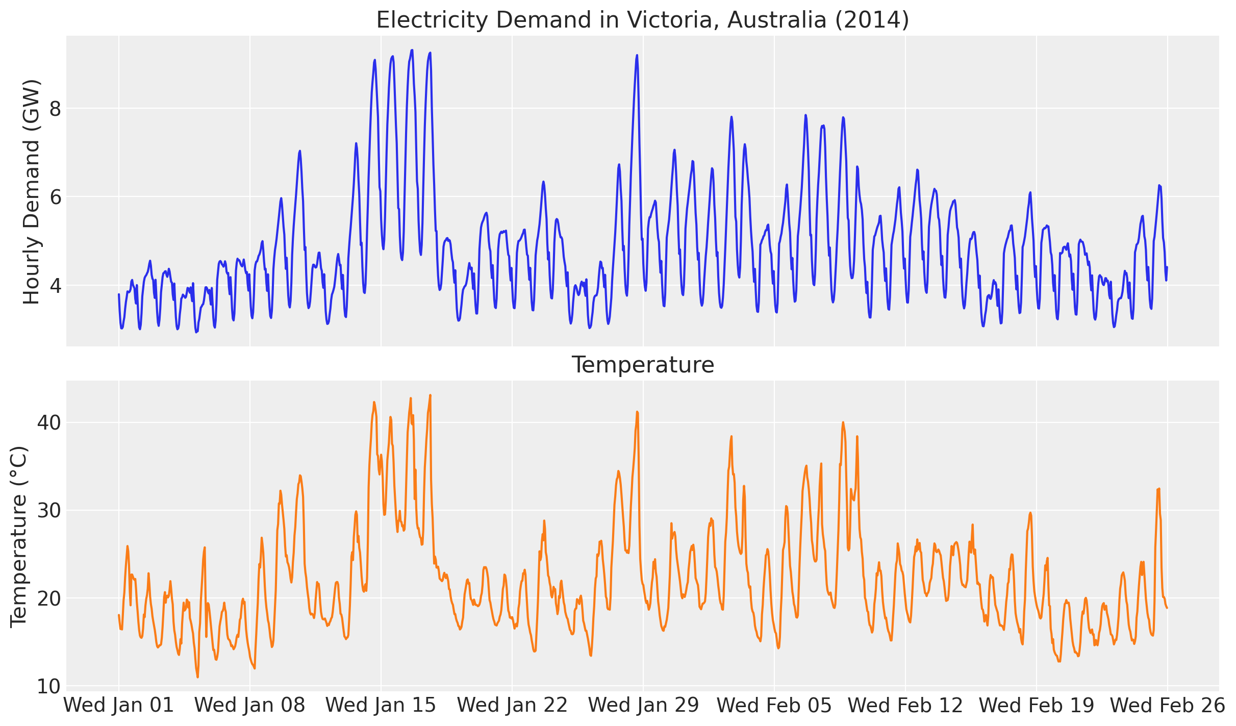
As a reminder, we are interested in a forecasting model where use temperature as a regressor. In addition, we want to understand the non-linear effect of temperature on demand.
Training and Test Data
To prepare the data for the model, we do a simple train-test split and create some seasonal features.
num_forecast_steps = 24 * 7 * 2  # Two weeks.
demand_training_data = demand[:-num_forecast_steps]
demand_test_data = demand[-num_forecast_steps:]

temperature_training_data = temperature[:-num_forecast_steps]
temperature_test_data = temperature[-num_forecast_steps:]

demand_dates_training_data = demand_dates[:-num_forecast_steps]
demand_dates_test_data = demand_dates[-num_forecast_steps:]

day_of_week = jnp.array([x.weekday() for x in demand_dates.astype(object)])
day_of_week_training_data = day_of_week[:-num_forecast_steps]
day_of_week_test_data = day_of_week[-num_forecast_steps:]


print(f"Demand training data shape: {demand_training_data.shape}")
print(f"Demand test data shape: {demand_test_data.shape}")
print(f"Temperature training data shape: {temperature_training_data.shape}")
print(f"Temperature test data shape: {temperature_test_data.shape}")
print(f"Day of week training data shape: {day_of_week_training_data.shape}")
print(f"Day of week test data shape: {day_of_week_test_data.shape}")
Demand training data shape: (1008,)
Demand test data shape: (336,)
Temperature training data shape: (1008,)
Temperature test data shape: (336,)
Day of week training data shape: (1008,)
Day of week test data shape: (336,)We can now visualize the training and test data of the demand.
fig, ax = plt.subplots()
ax.plot(demand_dates_training_data, demand_training_data, label="Training Data")
ax.plot(demand_dates_test_data, demand_test_data, label="Test Data")
ax.axvline(
    x=demand_dates_training_data[-1],
    color="black",
    linestyle="--",
    label="Training-Test Split",
)
ax.set(title="Demand Data", ylabel="Demand (GW)")
ax.legend()
ax.xaxis.set_major_locator(demand_loc)
ax.xaxis.set_major_formatter(demand_fmt);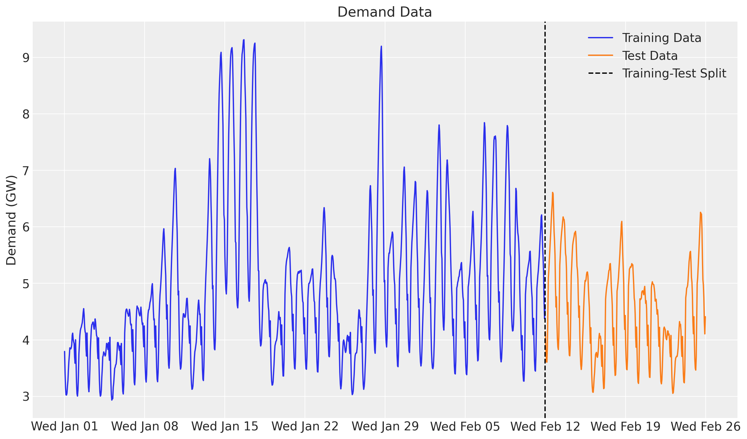
Model Specification
Here is a reminder of the base model components:
- We use a linear model to predict demand as a function of temperature and two seasonal effects: hour of day and day of week. We use Zero-Sum Normal distributions to model these seasonal effects.
- We use a Matérn 5/2 kernel to model the temperature effect on demand using the Hilbert Space Gaussian Process (HSGP) approximation from NumPyro (see here).
- The noise scale will vary with the temperature.
- We use a Student-t distribution to model the residual error.
For one of the seasonal components we need the next handy utility function:
def periodic_repeat_jax(tensor: Array, size: int, dim: int) -> Array:
    """
    Repeat a period-sized tensor up to given size using JAX.

    Parameters
    ----------
    tensor : Array
        A JAX array to be repeated.
    size : int
        Desired size of the result along dimension `dim`.
    dim : int
        The tensor dimension along which to repeat.

    Returns
    -------
    Array
        The repeated tensor.

    References
    ----------
    Thttps://docs.pyro.ai/en/stable/ops.html#pyro.ops.tensor_utils.periodic_repeat
    """
    assert isinstance(size, int) and size >= 0
    assert isinstance(dim, int)
    if dim >= 0:
        dim -= tensor.ndim

    period = tensor.shape[dim]
    repeats = [1] * tensor.ndim
    repeats[dim] = (size + period - 1) // period
    result = jnp.tile(tensor, repeats)

    slices = [slice(None)] * tensor.ndim
    slices[dim] = slice(None, size)

    return result[tuple(slices)]
Domain Knowledge Priors
Let us assume that we know from domain knowledge (science or a natural experiment, for example when the electricity system broke in a similar area and we could estimate lifts) that the effect of temperature on demand over \(32\)°C is somehow stable at around a value of \(0.13\). We believe this is useful information and in our previous baseline model the effect at this regime was increasing linearly from \(0.11\) to \(0.15\). The baseline still oscillates around the expected value of \(0.13\), but we want to make sure our effect is very conservative at this regime.
In order to do so, the idea presented in the Pyro example Forecasting with Dynamic Linear Model (DLM) is to add an additional an likelihood for the temperature range of interest where we set the latent effect variable as observed.
Let’s look into the details of this approach. The baseline model is exactly the same as in our example before Electricity Demand Forecast: Dynamic Time-Series Model.
# Set the temperature threshold for the prior
temperature_threshold_prior = 32.0

# Get the indices of the temperature data that is over the threshold
temperature_prior_idx = jnp.where(
    temperature_training_data > temperature_threshold_prior
)[0]
Now we are ready to specify the NumPyro model with the additional likelihood for the temperature prior.
def model(
    temperature: Float[Array, " t"],
    day_of_week: Int[Array, " t"],
    ell: float = 55.0,
    m: int = 25,
    temperature_prior_idx: Int[Array, " n_priors"] | None = None,
    demand: Float[Array, " t"] | None = None,
) -> None:
    t_max = temperature.size

    # Intercept
    intercept = numpyro.sample("intercept", dist.Normal(loc=0, scale=2))

    # GP Parameters
    ## Amplitude
    alpha = numpyro.sample("alpha", dist.InverseGamma(concentration=6.66, rate=1.57))
    ## Length Scale
    length_scale = numpyro.sample(
        "length_scale", dist.InverseGamma(concentration=11, rate=62.2)
    )
    ## Scale Factor
    scale_factor = numpyro.sample("scale", dist.HalfNormal(scale=0.5))
    ## Noise Scale
    # Degrees of Freedom for the Student-t distribution
    nu = numpyro.sample("nu", dist.Gamma(concentration=8, rate=3))

    # Temperature Effect as a HSGP
    beta_temperature = numpyro.deterministic(
        "beta_temperature",
        hsgp_matern(
            x=temperature,
            nu=5 / 2,
            alpha=alpha,
            length=length_scale,
            ell=ell,
            m=m,
        ),
    )

    # Hour of Day Effect
    scale_hour_of_day = numpyro.sample("scale_hour_of_day", dist.HalfNormal(scale=0.5))
    hour_of_day_effect = numpyro.sample(
        "hour_of_day_effect",
        dist.ZeroSumNormal(scale=scale_hour_of_day, event_shape=(24,)),
    )
    hour_of_day_effect_repeat = periodic_repeat_jax(hour_of_day_effect, t_max, dim=0)

    # Day of Week Effect
    scale_day_of_week = numpyro.sample("scale_day_of_week", dist.HalfNormal(scale=0.5))
    day_of_week_effect = numpyro.sample(
        "day_of_week_effect",
        dist.ZeroSumNormal(scale=scale_day_of_week, event_shape=(7,)),
    )

    # Add additional likelihood for the temperature prior
    # effect on demand for very hot days
    if temperature_prior_idx is not None:
        temperature_prior_effect_mean = 0.13
        temperature_prior_effect_scale = 0.01  # <- Uncertainty of the prior
        numpyro.sample(
            "temperature_prior",
            dist.Normal(
                loc=temperature_prior_effect_mean, scale=temperature_prior_effect_scale
            ),
            obs=beta_temperature[temperature_prior_idx],
        )
    # Expected Value
    mu = (
        intercept
        + beta_temperature * temperature
        + hour_of_day_effect_repeat
        + day_of_week_effect[day_of_week]
    )

    scale = scale_factor * jnp.sqrt(temperature)

    # Likelihood
    with numpyro.plate("data", t_max):
        numpyro.sample("obs", dist.StudentT(df=nu, loc=mu, scale=scale), obs=demand)
Since the model is exactly the same as in the previous example, we go directly to inference (even though we should always run the prior predictive checks).
Inference with SVI
We use stochastic variational inference to fit the model.
guide = AutoNormal(model)
optimizer = numpyro.optim.Adam(step_size=0.005)
svi = SVI(model, guide, optimizer, loss=Trace_ELBO())
num_steps = 50_000

rng_key, rng_subkey = random.split(key=rng_key)

svi_result = svi.run(
    rng_subkey,
    num_steps,
    temperature=temperature_training_data,
    day_of_week=day_of_week_training_data,
    temperature_prior_idx=temperature_prior_idx,
    demand=demand_training_data,
)

fig, ax = plt.subplots(figsize=(9, 6))
ax.plot(svi_result.losses)
ax.set_yscale("log")
ax.set_title("ELBO loss", fontsize=18, fontweight="bold");
100%|██████████| 50000/50000 [00:14<00:00, 3412.44it/s, init loss: 2701029.2500, avg. loss [47501-50000]: 446.1953]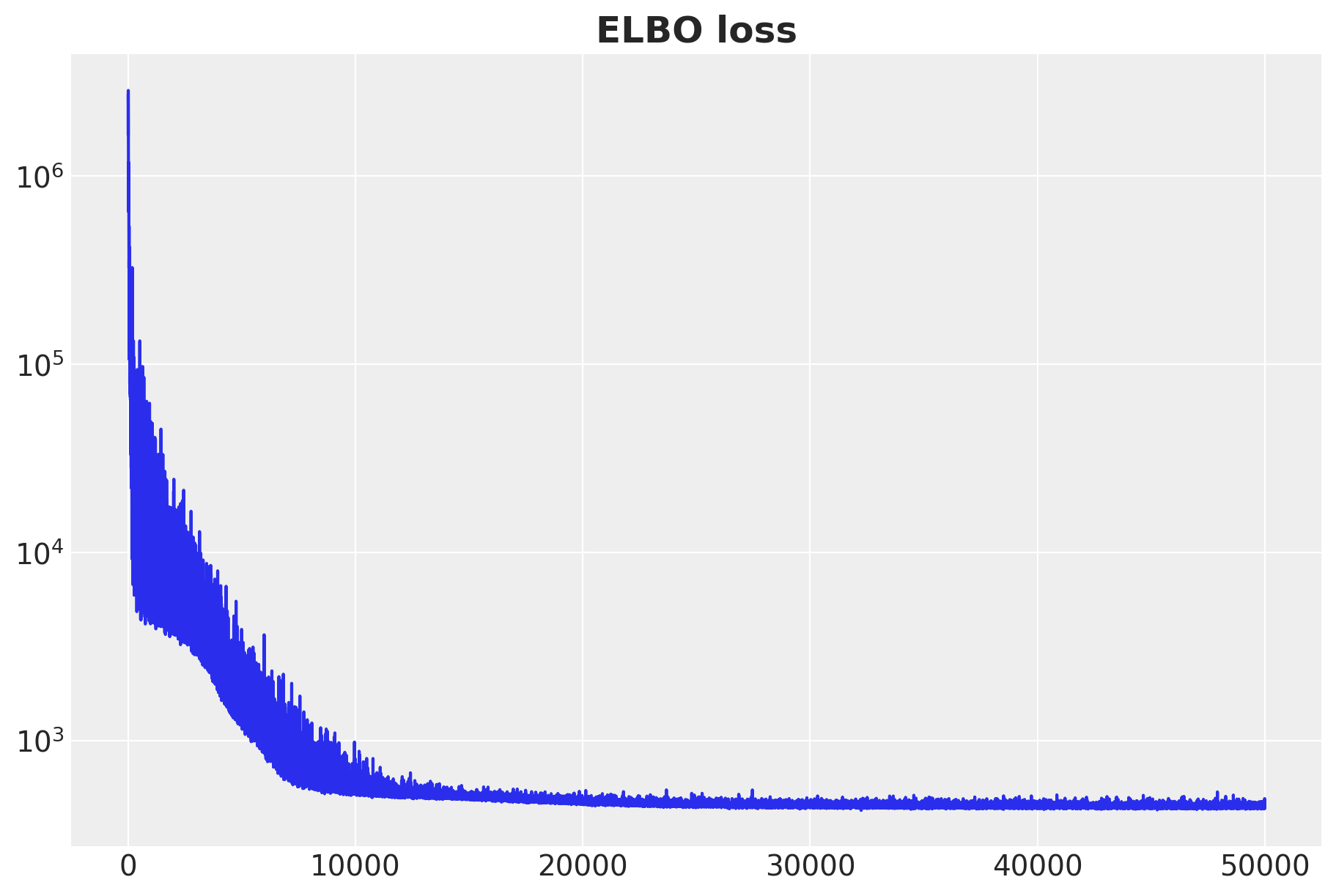
The ELBO loss is decreasing as expected.
Posterior Predictive Checks
We now collect the posterior samples for the in and out of sample data.
posterior = Predictive(
    model=model,
    guide=guide,
    params=svi_result.params,
    num_samples=5_000,
    return_sites=["beta_temperature", "obs"],
)

rng_key, rng_subkey = random.split(rng_key)
train_posterior_samples = posterior(
    rng_subkey,
    temperature=temperature_training_data,
    day_of_week=day_of_week_training_data,
    temperature_prior_idx=temperature_prior_idx,
)

rng_key, rng_subkey = random.split(rng_key)
test_posterior_samples = posterior(
    rng_subkey, temperature=temperature, day_of_week=day_of_week
)
idata_train = az.from_dict(
posterior={k: v[None, ...] for k, v in train_posterior_samples.items()},
coords={"time": demand_dates_training_data},
dims={"obs": ["time"], "beta_temperature": ["time"]},
)
idata_test = az.from_dict(
posterior={k: v[None, ...] for k, v in test_posterior_samples.items()},
coords={"time": demand_dates},
dims={"obs": ["time"], "beta_temperature": ["time"]},
)Forecast
We evaluate the forecast using the Continuous Ranked Probability Score (CRPS).
@jax.jit
def crps(
    truth: Float[Array, " t"],
    pred: Float[Array, "n_samples t"],
    sample_weight: Float[Array, " t"] | None = None,
) -> Float[Array, ""]:
    if pred.shape[1:] != (1,) * (pred.ndim - truth.ndim - 1) + truth.shape:
        raise ValueError(
            f"""Expected pred to have one extra sample dim on left.
            Actual shapes: {pred.shape} versus {truth.shape}"""
        )

    absolute_error = jnp.mean(jnp.abs(pred - truth), axis=0)

    num_samples = pred.shape[0]
    if num_samples == 1:
        return jnp.average(absolute_error, weights=sample_weight)

    pred = jnp.sort(pred, axis=0)
    diff = pred[1:] - pred[:-1]
    weight = jnp.arange(1, num_samples) * jnp.arange(num_samples - 1, 0, -1)
    weight = weight.reshape(weight.shape + (1,) * (diff.ndim - 1))

    per_obs_crps = absolute_error - jnp.sum(diff * weight, axis=0) / num_samples**2
    return jnp.average(per_obs_crps, weights=sample_weight)


crps_train = crps(
    demand_training_data, jnp.array(idata_train["posterior"]["obs"].sel(chain=0))
)

crps_test = crps(
    demand_test_data,
    jnp.array(
        idata_test["posterior"]["obs"]
        .sel(chain=0)
        .isel(time=slice(demand_dates_training_data.size, None))
    ),
)
We can now compare the posterior predictive distribution with the training and test data.
fig, ax = plt.subplots()

az.plot_hdi(
    demand_dates_training_data,
    idata_train["posterior"]["obs"],
    hdi_prob=0.94,
    smooth=False,
    color="C0",
    fill_kwargs={"alpha": 0.2, "label": "94% HDI"},
    ax=ax,
)

az.plot_hdi(
    demand_dates_training_data,
    idata_train["posterior"]["obs"],
    hdi_prob=0.5,
    smooth=False,
    color="C0",
    fill_kwargs={"alpha": 0.4, "label": "50% HDI"},
    ax=ax,
)

ax.plot(
    demand_dates_training_data,
    idata_train["posterior"]["obs"].mean(dim=("chain", "draw")),
    c="C0",
    label="Posterior Mean",
)

az.plot_hdi(
    demand_dates_test_data,
    idata_test["posterior"]["obs"].isel(
        time=slice(demand_dates_training_data.size, None)
    ),
    hdi_prob=0.94,
    smooth=False,
    color="C1",
    fill_kwargs={"alpha": 0.2, "label": "94% HDI"},
    ax=ax,
)

az.plot_hdi(
    demand_dates_test_data,
    idata_test["posterior"]["obs"].isel(
        time=slice(demand_dates_training_data.size, None)
    ),
    hdi_prob=0.5,
    smooth=False,
    color="C1",
    fill_kwargs={"alpha": 0.4, "label": "50% HDI"},
    ax=ax,
)

ax.plot(
    demand_dates_test_data,
    idata_test["posterior"]["obs"]
    .isel(time=slice(demand_dates_training_data.size, None))
    .mean(dim=("chain", "draw")),
    c="C1",
    label="Posterior Mean",
)

ax.plot(
    demand_dates_training_data, demand_training_data, c="black", label="Training Data"
)

ax.plot(demand_dates_test_data, demand_test_data, c="black", label="Test Data")

ax.legend(loc="upper center", bbox_to_anchor=(0.5, -0.1), ncol=4)
ax.set(
    title=f"Train CRPS: {crps_train:.3f}, Test CRPS: {crps_test:.3f}",
    ylabel="Demand (GW)",
    xlabel="Time",
)
ax.xaxis.set_major_locator(demand_loc)
ax.xaxis.set_major_formatter(demand_fmt)

fig.suptitle("Posterior Predictive Checks", fontsize=18, fontweight="bold");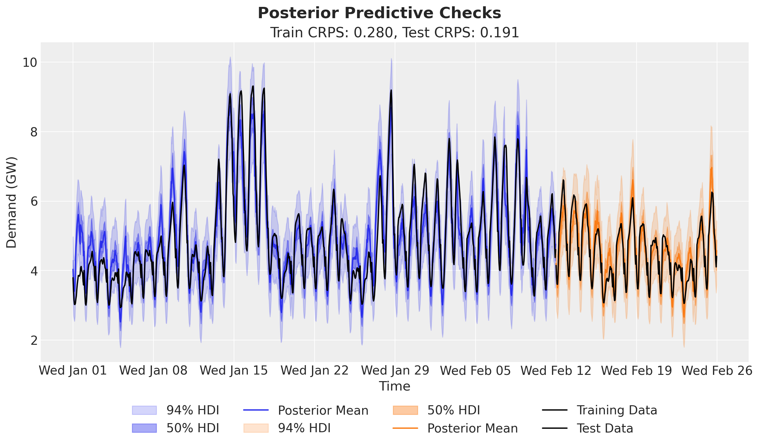
The forecasting metrics are pretty much the same as in the previous uncalibrated model (a really minor difference).
Temperature Effect on Demand
finally, let’s plot the temperature effect on demand.
temperature_prior_effect_mean = 0.13
temperature_prior_effect_scale = 0.01

fig, ax = plt.subplots()

az.plot_hdi(
    temperature_training_data,
    idata_train["posterior"]["beta_temperature"],
    hdi_prob=0.94,
    smooth=True,
    color="C1",
    fill_kwargs={"alpha": 0.3, "label": "94% HDI"},
    ax=ax,
)

az.plot_hdi(
    temperature_training_data,
    idata_train["posterior"]["beta_temperature"],
    hdi_prob=0.5,
    smooth=True,
    color="C1",
    fill_kwargs={"alpha": 0.5, "label": "50% HDI"},
    ax=ax,
)

ax.axvline(
    temperature_threshold_prior,
    c="black",
    linestyle="--",
    label="Temperature Threshold Prior",
)

ax.axhspan(
    ymin=temperature_prior_effect_mean - 1 * temperature_prior_effect_scale,
    ymax=temperature_prior_effect_mean + 1 * temperature_prior_effect_scale,
    xmin=0.64,
    xmax=1,
    color="C3",
    alpha=0.1,
    label="Temperature Prior Effect Band (1 std)",
)
ax.axhline(
    temperature_prior_effect_mean,
    c="C3",
    linestyle="--",
    label="Temperature Prior Effect Mean",
)
ax.legend(loc="lower center", bbox_to_anchor=(0.5, -0.25), ncol=3)
ax.set(
    title="Temperature Effect on Demand",
    xlabel="Temperature (°C)",
    ylabel="Effect on Demand",
);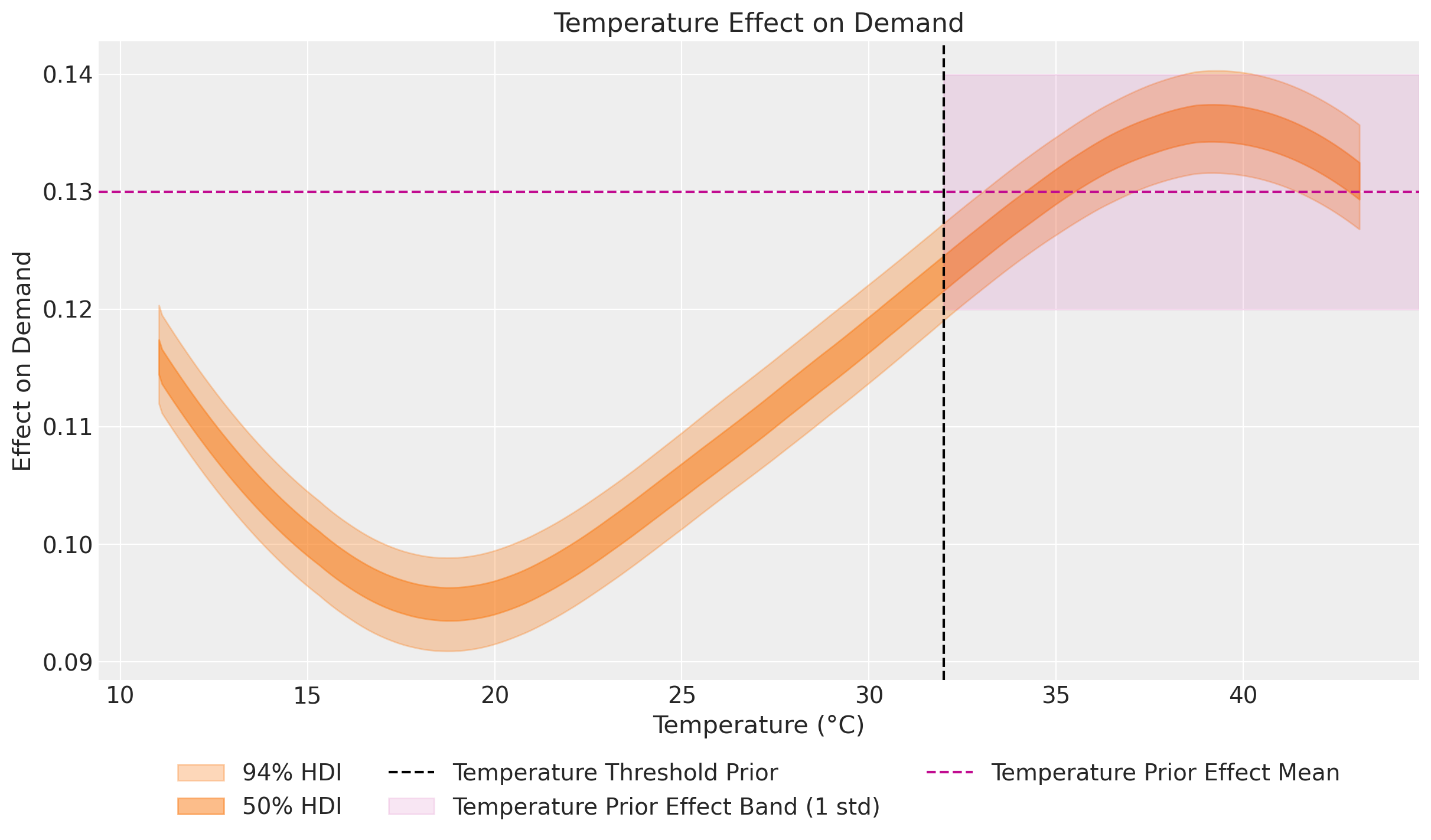
The overall shape of the curve resembles the one in the previous baseline uncalibrated model. Still, we see that the effect of the priors is making the estimate for temperatures over \(32\)°C to be more conservative around the expected value of \(0.13\).
Observe that this opens great opportunities to calibrate forecasting models with domain knowledge, possible extracted from experimental or observational data.