We work out a classical electricity demand forecasting model form the case study Structural Time Series Modeling Case Studies: Atmospheric CO2 and Electricity Demand from the TensorFlow Probability documentation. The idea of this example is to use temperature as a linear covariate to model the electricity demand. In this example, we show how to use a (Hilbert Space Approximation) Gaussian process to model the non-linear relationship between temperature and electricity demand (for an introduction to the topic see A Conceptual and Practical Introduction to Hilbert Space GPs Approximation Methods). This technique improves the simple linear model in and out of sample predictions as we aro not using the Gaussian process to extrapolate over time, but rather to model the non-linear relationship between temperature and electricity demand, similarly as how it has done in the example Time-Varying Regression Coefficients via Hilbert Space Gaussian Process Approximation.
Prepare Notebook
import arviz as az
import jax
import jax.numpy as jnp
import matplotlib.dates as mdates
import matplotlib.pyplot as plt
import numpy as np
import numpyro
import numpyro.distributions as dist
import preliz as pz
from jax import random
from jaxtyping import Array, Float, Int
from numpyro.contrib.hsgp.approximation import hsgp_matern
from numpyro.infer import SVI, Predictive, Trace_ELBO
from numpyro.infer.autoguide import AutoNormal

az.style.use("arviz-darkgrid")
plt.rcParams["figure.figsize"] = [12, 7]
plt.rcParams["figure.dpi"] = 100
plt.rcParams["figure.facecolor"] = "white"

numpyro.set_host_device_count(n=4)

rng_key = random.PRNGKey(seed=42)

%load_ext autoreload
%autoreload 2
%load_ext jaxtyping
%jaxtyping.typechecker beartype.beartype
%config InlineBackend.figure_format = "retina"
Load Data
We load the data explicitly as in the Tensorflow Probability example. We reference the original comment:
“Victoria electricity demand dataset, as presented at https://otexts.com/fpp2/scatterplots.html and downloaded from https://github.com/robjhyndman/fpp2-package/blob/master/data/elecdaily.rda . This series contains the first eight weeks (starting Jan 1). The original dataset was half-hourly data; here we’ve downsampled to hourly data by taking every other timestep.”
demand_dates = np.arange("2014-01-01", "2014-02-26", dtype="datetime64[h]")
demand_loc = mdates.WeekdayLocator(byweekday=mdates.WE)
demand_fmt = mdates.DateFormatter("%a %b %d")

demand = jnp.array(
    np.array(
        "3.794,3.418,3.152,3.026,3.022,3.055,3.180,3.276,3.467,3.620,3.730,3.858,3.851,3.839,3.861,3.912,4.082,4.118,4.011,3.965,3.932,3.693,3.585,4.001,3.623,3.249,3.047,3.004,3.104,3.361,3.749,3.910,4.075,4.165,4.202,4.225,4.265,4.301,4.381,4.484,4.552,4.440,4.233,4.145,4.116,3.831,3.712,4.121,3.764,3.394,3.159,3.081,3.216,3.468,3.838,4.012,4.183,4.269,4.280,4.310,4.315,4.233,4.188,4.263,4.370,4.308,4.182,4.075,4.057,3.791,3.667,4.036,3.636,3.283,3.073,3.003,3.023,3.113,3.335,3.484,3.697,3.723,3.786,3.763,3.748,3.714,3.737,3.828,3.937,3.929,3.877,3.829,3.950,3.756,3.638,4.045,3.682,3.283,3.036,2.933,2.956,2.959,3.157,3.236,3.370,3.493,3.516,3.555,3.570,3.656,3.792,3.950,3.953,3.926,3.849,3.813,3.891,3.683,3.562,3.936,3.602,3.271,3.085,3.041,3.201,3.570,4.123,4.307,4.481,4.533,4.545,4.524,4.470,4.457,4.418,4.453,4.539,4.473,4.301,4.260,4.276,3.958,3.796,4.180,3.843,3.465,3.246,3.203,3.360,3.808,4.328,4.509,4.598,4.562,4.566,4.532,4.477,4.442,4.424,4.486,4.579,4.466,4.338,4.270,4.296,4.034,3.877,4.246,3.883,3.520,3.306,3.252,3.387,3.784,4.335,4.465,4.529,4.536,4.589,4.660,4.691,4.747,4.819,4.950,4.994,4.798,4.540,4.352,4.370,4.047,3.870,4.245,3.848,3.509,3.302,3.258,3.419,3.809,4.363,4.605,4.793,4.908,5.040,5.204,5.358,5.538,5.708,5.888,5.966,5.817,5.571,5.321,5.141,4.686,4.367,4.618,4.158,3.771,3.555,3.497,3.646,4.053,4.687,5.052,5.342,5.586,5.808,6.038,6.296,6.548,6.787,6.982,7.035,6.855,6.561,6.181,5.899,5.304,4.795,4.862,4.264,3.820,3.588,3.481,3.514,3.632,3.857,4.116,4.375,4.462,4.460,4.422,4.398,4.407,4.480,4.621,4.732,4.735,4.572,4.385,4.323,4.069,3.940,4.247,3.821,3.416,3.220,3.124,3.132,3.181,3.337,3.469,3.668,3.788,3.834,3.894,3.964,4.109,4.275,4.472,4.623,4.703,4.594,4.447,4.459,4.137,3.913,4.231,3.833,3.475,3.302,3.279,3.519,3.975,4.600,4.864,5.104,5.308,5.542,5.759,6.005,6.285,6.617,6.993,7.207,7.095,6.839,6.387,6.048,5.433,4.904,4.959,4.425,4.053,3.843,3.823,4.017,4.521,5.229,5.802,6.449,6.975,7.506,7.973,8.359,8.596,8.794,9.030,9.090,8.885,8.525,8.147,7.797,6.938,6.215,6.123,5.495,5.140,4.896,4.812,5.024,5.536,6.293,7.000,7.633,8.030,8.459,8.768,9.000,9.113,9.155,9.173,9.039,8.606,8.095,7.617,7.208,6.448,5.740,5.718,5.106,4.763,4.610,4.566,4.737,5.204,5.988,6.698,7.438,8.040,8.484,8.837,9.052,9.114,9.214,9.307,9.313,9.006,8.556,8.275,7.911,7.077,6.348,6.175,5.455,5.041,4.759,4.683,4.908,5.411,6.199,6.923,7.593,8.090,8.497,8.843,9.058,9.159,9.231,9.253,8.852,7.994,7.388,6.735,6.264,5.690,5.227,5.220,4.593,4.213,3.984,3.891,3.919,4.031,4.287,4.558,4.872,4.963,5.004,5.017,5.057,5.064,5.000,5.023,5.007,4.923,4.740,4.586,4.517,4.236,4.055,4.337,3.848,3.473,3.273,3.198,3.204,3.252,3.404,3.560,3.767,3.896,3.934,3.972,3.985,4.032,4.122,4.239,4.389,4.499,4.406,4.356,4.396,4.106,3.914,4.265,3.862,3.546,3.360,3.359,3.649,4.180,4.813,5.086,5.301,5.384,5.434,5.470,5.529,5.582,5.618,5.636,5.561,5.291,5.000,4.840,4.767,4.364,4.160,4.452,4.011,3.673,3.503,3.483,3.695,4.213,4.810,5.028,5.149,5.182,5.208,5.179,5.190,5.220,5.202,5.216,5.232,5.019,4.828,4.686,4.657,4.304,4.106,4.389,3.955,3.643,3.489,3.479,3.695,4.187,4.732,4.898,4.997,5.001,5.022,5.052,5.094,5.143,5.178,5.250,5.255,5.075,4.867,4.691,4.665,4.352,4.121,4.391,3.966,3.615,3.437,3.430,3.666,4.149,4.674,4.851,5.011,5.105,5.242,5.378,5.576,5.790,6.030,6.254,6.340,6.253,6.039,5.736,5.490,4.936,4.580,4.742,4.230,3.895,3.712,3.700,3.906,4.364,4.962,5.261,5.463,5.495,5.477,5.394,5.250,5.159,5.081,5.083,5.038,4.857,4.643,4.526,4.428,4.141,3.975,4.290,3.809,3.423,3.217,3.132,3.192,3.343,3.606,3.803,3.963,3.998,3.962,3.894,3.814,3.776,3.808,3.914,4.033,4.079,4.027,3.974,4.057,3.859,3.759,4.132,3.716,3.325,3.111,3.030,3.046,3.096,3.254,3.390,3.606,3.718,3.755,3.768,3.768,3.834,3.957,4.199,4.393,4.532,4.516,4.380,4.390,4.142,3.954,4.233,3.795,3.425,3.209,3.124,3.177,3.288,3.498,3.715,4.092,4.383,4.644,4.909,5.184,5.518,5.889,6.288,6.643,6.729,6.567,6.179,5.903,5.278,4.788,4.885,4.363,4.011,3.823,3.762,3.998,4.598,5.349,5.898,6.487,6.941,7.381,7.796,8.185,8.522,8.825,9.103,9.198,8.889,8.174,7.214,6.481,5.611,5.026,5.052,4.484,4.148,3.955,3.873,4.060,4.626,5.272,5.441,5.535,5.534,5.610,5.671,5.724,5.793,5.838,5.908,5.868,5.574,5.276,5.065,4.976,4.554,4.282,4.547,4.053,3.720,3.536,3.524,3.792,4.420,5.075,5.208,5.344,5.482,5.701,5.936,6.210,6.462,6.683,6.979,7.059,6.893,6.535,6.121,5.797,5.152,4.705,4.805,4.272,3.975,3.805,3.775,3.996,4.535,5.275,5.509,5.730,5.870,6.034,6.175,6.340,6.500,6.603,6.804,6.787,6.460,6.043,5.627,5.367,4.866,4.575,4.728,4.157,3.795,3.607,3.537,3.596,3.803,4.125,4.398,4.660,4.853,5.115,5.412,5.669,5.930,6.216,6.466,6.641,6.605,6.316,5.821,5.520,5.016,4.657,4.746,4.197,3.823,3.613,3.505,3.488,3.532,3.716,4.011,4.421,4.836,5.296,5.766,6.233,6.646,7.011,7.380,7.660,7.804,7.691,7.364,7.019,6.260,5.545,5.437,4.806,4.457,4.235,4.172,4.396,5.002,5.817,6.266,6.732,7.049,7.184,7.085,6.798,6.632,6.408,6.218,5.968,5.544,5.217,4.964,4.758,4.328,4.074,4.367,3.883,3.536,3.404,3.396,3.624,4.271,4.916,4.953,5.016,5.048,5.106,5.124,5.200,5.244,5.242,5.341,5.368,5.166,4.910,4.762,4.700,4.276,4.035,4.318,3.858,3.550,3.399,3.382,3.590,4.261,4.937,4.994,5.094,5.168,5.303,5.410,5.571,5.740,5.900,6.177,6.274,6.039,5.700,5.389,5.192,4.672,4.359,4.614,4.118,3.805,3.627,3.646,3.882,4.470,5.106,5.274,5.507,5.711,5.950,6.200,6.527,6.884,7.196,7.615,7.845,7.759,7.437,7.059,6.584,5.742,5.125,5.139,4.564,4.218,4.025,4.000,4.245,4.783,5.504,5.920,6.271,6.549,6.894,7.231,7.535,7.597,7.562,7.609,7.534,7.118,6.448,5.963,5.565,5.005,4.666,4.850,4.302,3.905,3.678,3.610,3.672,3.869,4.204,4.541,4.944,5.265,5.651,6.090,6.547,6.935,7.318,7.625,7.793,7.760,7.510,7.145,6.805,6.103,5.520,5.462,4.824,4.444,4.237,4.157,4.164,4.275,4.545,5.033,5.594,6.176,6.681,6.628,6.238,6.039,5.897,5.832,5.701,5.483,4.949,4.589,4.407,4.027,3.820,4.075,3.650,3.388,3.271,3.268,3.498,4.086,4.800,4.933,5.102,5.126,5.194,5.260,5.319,5.364,5.419,5.559,5.568,5.332,5.027,4.864,4.738,4.303,4.093,4.379,3.952,3.632,3.461,3.446,3.732,4.294,4.911,5.021,5.138,5.223,5.348,5.479,5.661,5.832,5.966,6.178,6.212,5.949,5.640,5.449,5.213,4.678,4.376,4.601,4.147,3.815,3.610,3.605,3.879,4.468,5.090,5.226,5.406,5.561,5.740,5.899,6.095,6.272,6.402,6.610,6.585,6.265,5.925,5.747,5.497,4.932,4.580,4.763,4.298,4.026,3.871,3.827,4.065,4.643,5.317,5.494,5.685,5.814,5.912,5.999,6.097,6.176,6.136,6.131,6.049,5.796,5.532,5.475,5.254,4.742,4.453,4.660,4.176,3.895,3.726,3.717,3.910,4.479,5.135,5.306,5.520,5.672,5.737,5.785,5.829,5.893,5.892,5.921,5.817,5.557,5.304,5.234,5.074,4.656,4.396,4.599,4.064,3.749,3.560,3.475,3.552,3.783,4.045,4.258,4.539,4.762,4.938,5.049,5.037,5.066,5.151,5.197,5.201,5.132,4.908,4.725,4.568,4.222,3.939,4.215,3.741,3.380,3.174,3.076,3.071,3.172,3.328,3.427,3.603,3.738,3.765,3.777,3.705,3.690,3.742,3.859,4.032,4.113,4.032,4.066,4.011,3.712,3.530,3.905,3.556,3.283,3.136,3.146,3.400,4.009,4.717,4.827,4.909,4.973,5.036,5.079,5.160,5.228,5.241,5.343,5.350,5.184,4.941,4.797,4.615,4.160,3.904,4.213,3.810,3.528,3.369,3.381,3.609,4.178,4.861,4.918,5.006,5.102,5.239,5.385,5.528,5.724,5.845,6.048,6.097,5.838,5.507,5.267,5.003,4.462,4.184,4.431,3.969,3.660,3.480,3.470,3.693,4.313,4.955,5.083,5.251,5.268,5.293,5.285,5.308,5.349,5.322,5.328,5.151,4.975,4.741,4.678,4.458,4.056,3.868,4.226,3.799,3.428,3.253,3.228,3.452,4.040,4.726,4.709,4.721,4.741,4.846,4.864,4.868,4.836,4.799,4.890,4.946,4.800,4.646,4.693,4.546,4.117,3.897,4.259,3.893,3.505,3.341,3.334,3.623,4.240,4.925,4.986,5.028,4.987,4.984,4.975,4.912,4.833,4.686,4.710,4.718,4.577,4.454,4.532,4.407,4.064,3.883,4.221,3.792,3.445,3.261,3.221,3.295,3.521,3.804,4.038,4.200,4.226,4.198,4.182,4.078,4.018,4.002,4.066,4.158,4.154,4.084,4.104,4.001,3.773,3.700,4.078,3.702,3.349,3.143,3.052,3.070,3.181,3.327,3.440,3.616,3.678,3.694,3.710,3.706,3.764,3.852,4.009,4.202,4.323,4.249,4.275,4.162,3.848,3.706,4.060,3.703,3.401,3.251,3.239,3.455,4.041,4.743,4.815,4.916,4.931,4.966,5.063,5.218,5.381,5.458,5.550,5.566,5.376,5.104,5.022,4.793,4.335,4.108,4.410,4.008,3.666,3.497,3.464,3.698,4.333,4.998,5.094,5.272,5.459,5.648,5.853,6.062,6.258,6.236,6.226,5.957,5.455,5.066,4.968,4.742,4.304,4.105,4.410".split(
            ","
        )
    ).astype(np.float32)
)

temperature = jnp.array(
    np.array(
        "18.050,17.200,16.450,16.650,16.400,17.950,19.700,20.600,22.350,23.700,24.800,25.900,25.300,23.650,20.700,19.150,22.650,22.650,22.400,22.150,22.050,22.150,21.000,19.500,18.450,17.250,16.300,15.700,15.500,15.450,15.650,16.500,18.100,17.800,19.100,19.850,20.300,21.050,22.800,21.650,20.150,19.300,18.750,17.900,17.350,16.850,16.350,15.700,14.950,14.500,14.350,14.450,14.600,14.600,14.700,15.450,16.700,18.300,20.100,20.650,19.450,20.200,20.250,20.050,20.250,20.950,21.900,21.000,19.900,19.250,17.300,16.300,15.800,15.000,14.400,14.050,13.650,13.500,14.150,15.300,14.800,17.050,18.350,19.450,18.550,18.650,18.850,19.800,19.650,18.900,19.500,17.700,17.350,16.950,16.400,15.950,14.900,14.250,13.050,12.000,11.500,10.950,12.300,16.100,17.100,19.600,21.100,22.600,24.350,25.250,25.750,20.350,15.550,18.300,19.400,19.250,18.550,17.700,16.750,15.800,14.900,14.050,14.100,13.500,13.000,12.950,13.300,13.900,15.400,16.750,17.300,17.750,18.400,18.500,18.800,19.450,18.750,18.400,16.950,15.800,15.350,15.250,15.150,14.900,14.500,14.600,14.400,14.150,14.300,14.500,14.950,15.550,15.800,15.550,16.450,17.500,17.700,18.750,19.600,19.900,19.350,19.550,17.900,16.400,15.550,14.900,14.400,13.950,13.300,12.950,12.650,12.450,12.350,12.150,11.950,14.150,15.850,17.750,19.450,22.150,23.850,23.450,24.950,26.850,26.100,25.150,23.250,21.300,19.850,18.900,18.250,17.450,17.100,16.400,15.550,15.050,14.400,14.550,15.150,17.050,18.850,20.850,24.250,27.700,28.400,30.750,30.700,32.200,31.750,30.650,29.750,28.850,27.850,25.950,24.700,24.850,24.050,23.850,23.500,22.950,22.200,21.750,22.350,24.050,25.150,27.100,28.050,29.750,31.250,31.900,32.950,33.150,33.950,33.850,33.250,32.500,31.500,28.300,23.900,22.900,22.300,21.250,20.500,19.850,18.850,18.300,18.100,18.200,18.150,18.000,17.700,18.250,19.700,20.750,21.800,21.500,21.600,20.800,19.400,18.400,17.900,17.600,17.550,17.550,17.650,17.400,17.150,16.800,17.000,16.900,17.200,17.350,17.650,17.800,18.400,19.300,20.200,21.050,21.700,21.800,21.800,21.500,20.000,19.300,18.200,18.100,17.700,16.950,16.250,15.600,15.500,15.300,15.450,15.500,15.750,17.350,19.150,21.650,24.700,25.200,24.300,26.900,28.100,29.450,29.850,29.450,26.350,27.050,25.700,25.150,23.850,22.450,21.450,20.850,20.700,21.300,21.550,20.800,22.300,26.300,32.600,35.150,36.800,38.150,39.950,40.850,41.250,42.300,41.950,41.350,40.600,36.350,36.150,34.600,34.050,35.400,36.300,35.550,33.700,30.650,29.450,29.500,31.000,33.300,35.700,36.650,37.650,39.400,40.600,40.250,37.550,37.300,35.400,32.750,31.200,29.600,28.350,27.500,28.750,28.900,29.900,28.700,28.650,28.150,28.250,27.650,27.800,29.450,32.500,35.750,38.850,39.900,41.100,41.800,42.750,39.900,39.750,40.800,37.950,31.250,34.600,30.250,28.500,27.900,27.950,27.300,26.900,26.800,26.050,26.100,27.700,31.850,34.850,36.350,38.000,39.200,41.050,41.600,42.350,43.100,33.500,30.700,29.100,26.400,23.900,24.700,24.350,23.450,23.450,23.550,23.050,22.200,22.100,22.000,21.900,22.050,22.550,22.850,22.450,22.250,22.650,22.350,21.900,21.000,20.950,20.200,19.700,19.400,19.200,18.650,18.150,18.150,17.650,17.350,17.150,16.800,16.750,16.400,16.500,16.700,17.300,17.750,19.200,20.400,20.900,21.450,22.000,22.100,21.600,21.700,20.500,19.850,19.750,19.500,19.200,19.800,19.500,19.200,19.200,19.150,19.050,19.100,19.250,19.550,20.200,20.550,21.450,23.150,23.500,23.400,23.500,23.300,22.850,22.250,20.950,19.750,19.450,18.900,18.450,17.950,17.550,17.300,16.950,16.900,16.850,17.100,17.250,17.400,17.850,18.100,18.600,19.700,21.000,21.400,22.650,22.550,22.000,21.050,19.550,18.550,18.300,17.750,17.800,17.650,17.800,17.450,16.950,16.500,16.900,17.050,16.750,17.300,18.800,19.350,20.750,21.400,21.900,21.950,22.800,22.750,23.200,22.650,20.800,19.250,17.800,16.950,16.550,16.050,15.750,15.150,14.700,14.150,13.900,13.900,14.000,15.800,17.650,19.700,22.500,25.300,24.300,24.650,26.450,27.250,26.550,28.800,27.850,25.200,24.750,23.750,22.550,22.350,21.700,21.300,20.300,20.050,20.500,21.250,20.850,21.000,19.400,18.900,18.150,18.650,20.200,20.000,21.650,21.950,21.150,20.400,19.500,19.150,18.400,18.050,17.750,17.600,17.150,16.750,16.350,16.250,15.900,15.850,15.900,16.200,18.500,18.750,18.800,19.850,19.750,19.600,19.300,20.000,20.250,19.700,18.600,17.400,17.100,16.650,16.250,16.250,15.800,15.350,14.800,14.250,13.500,13.400,14.350,15.800,17.700,19.000,21.050,22.200,22.450,24.950,24.750,25.050,26.400,26.200,26.500,25.850,24.400,23.600,22.650,21.500,20.150,19.900,18.850,18.700,18.750,18.650,20.050,23.450,24.900,26.450,28.550,30.600,31.550,32.800,33.500,33.700,34.450,34.200,33.650,32.900,31.750,30.500,29.250,28.100,26.450,25.400,25.400,25.150,25.400,25.100,25.950,28.100,30.400,32.000,33.750,34.700,35.800,37.000,39.050,39.750,41.200,41.050,36.050,28.250,24.450,23.150,22.050,21.600,21.450,20.800,20.250,19.700,19.400,19.650,19.100,18.650,18.900,19.400,20.700,21.750,22.350,24.100,23.350,24.400,22.950,22.400,20.950,19.600,18.900,18.000,17.400,16.800,16.550,16.300,16.250,16.750,16.700,17.100,17.500,18.150,18.850,20.650,22.600,25.600,28.500,26.750,27.200,27.300,27.500,27.000,25.450,24.500,23.850,23.200,22.550,21.850,21.050,20.200,19.950,20.400,20.300,20.100,20.450,20.900,21.450,21.800,23.250,24.100,25.200,25.550,25.900,25.450,26.050,25.350,23.900,22.250,22.000,21.700,21.450,20.550,19.000,18.850,18.700,19.050,19.350,19.350,19.450,19.600,20.550,22.400,24.550,26.900,27.950,28.500,28.200,29.050,28.700,28.800,27.150,24.900,23.500,23.350,23.000,22.300,21.400,20.700,19.850,19.400,19.250,18.700,18.650,20.200,23.400,26.400,27.450,29.150,32.050,34.500,34.950,36.550,37.850,38.400,35.150,34.050,34.100,33.100,30.300,29.300,27.550,26.600,25.900,25.500,25.150,25.000,25.150,27.000,31.150,32.750,31.500,26.900,23.900,23.150,22.850,21.500,21.150,21.300,19.700,18.800,18.450,18.300,17.800,16.850,16.400,16.150,15.700,15.500,15.400,15.300,15.050,15.650,18.100,19.200,21.050,22.350,23.450,24.850,24.950,25.550,25.300,24.250,22.750,20.850,19.350,18.250,17.450,17.000,16.500,16.100,15.950,15.300,14.550,14.250,14.400,15.550,18.300,20.000,22.750,25.450,25.800,26.350,29.150,30.450,30.350,29.600,27.550,25.550,23.650,22.950,21.850,20.700,20.150,19.300,19.000,18.400,17.800,17.750,18.000,20.800,23.400,25.750,27.750,29.600,32.150,32.900,33.650,34.300,34.800,35.050,33.750,33.250,32.400,31.250,29.650,28.550,26.550,25.950,25.000,24.400,24.150,24.150,24.350,26.900,28.750,30.350,32.750,34.250,35.300,28.400,27.250,26.600,25.750,25.350,23.150,21.550,20.850,20.550,20.350,20.550,20.600,19.900,19.550,19.200,18.900,18.850,19.250,21.000,23.050,25.350,27.700,31.050,35.250,35.100,36.850,39.250,40.000,39.450,38.950,37.750,33.850,30.400,25.700,25.400,25.600,28.150,32.400,31.850,31.350,31.200,31.100,31.950,32.450,35.200,38.400,35.850,30.700,27.850,26.900,26.650,25.250,24.450,22.500,22.050,20.000,19.750,19.100,18.500,18.400,17.400,16.900,16.800,16.450,16.050,16.300,17.450,19.300,20.000,21.050,22.800,22.550,23.300,24.050,23.100,23.100,22.500,20.800,19.550,18.800,18.200,17.650,17.750,17.150,16.550,16.200,16.000,15.600,15.150,15.150,16.250,17.800,19.150,21.000,22.800,23.850,24.250,26.200,25.650,25.050,23.850,23.600,23.100,22.950,22.550,21.550,20.450,19.600,18.700,18.300,18.000,17.550,17.300,17.200,17.950,19.450,21.100,23.050,24.650,25.050,25.850,25.300,26.650,25.500,25.900,26.250,25.300,25.150,23.600,22.050,21.700,21.150,20.550,20.500,20.200,20.500,20.600,20.900,21.700,22.000,22.250,23.400,23.900,25.250,26.200,26.000,25.300,25.200,25.300,25.500,25.350,25.050,24.850,24.050,23.150,22.300,21.900,21.150,20.300,19.650,19.700,19.750,20.250,21.500,23.600,24.600,25.900,25.450,24.850,25.900,26.150,26.250,26.350,26.250,25.850,25.300,24.600,23.750,22.250,21.750,21.450,21.500,21.300,21.250,21.200,21.600,22.000,23.650,25.200,26.400,25.500,25.150,26.950,28.350,25.650,25.000,25.500,24.150,22.900,21.600,21.750,21.500,21.550,20.450,19.500,18.750,18.650,18.200,17.300,17.900,18.050,17.400,16.850,17.950,20.550,21.950,22.600,22.300,22.400,22.300,21.100,20.250,19.200,18.900,18.600,18.350,17.700,17.200,16.850,16.900,16.800,16.800,16.600,16.350,17.200,18.350,19.550,20.300,21.600,21.800,23.300,23.200,24.550,24.950,24.900,23.700,22.000,19.650,18.250,17.700,17.250,16.900,16.550,16.050,16.450,15.400,14.900,14.700,16.100,18.450,19.800,23.000,25.250,27.600,27.900,28.550,29.450,29.700,29.350,27.000,23.550,21.900,20.750,20.150,19.600,19.150,18.800,18.550,18.200,17.750,17.650,17.800,18.750,19.600,20.450,21.950,23.700,23.150,24.150,24.550,21.400,19.150,19.050,16.500,15.900,14.850,15.300,14.100,13.800,13.600,13.450,13.400,13.050,12.750,12.800,12.750,13.600,14.950,16.100,17.500,18.500,19.300,19.400,19.750,19.400,19.450,19.450,18.900,17.650,16.800,15.900,15.050,14.550,14.250,13.800,13.850,13.700,13.650,13.350,13.400,14.050,15.000,16.650,17.850,18.450,18.200,18.900,19.850,20.000,19.700,18.800,17.500,16.600,16.250,16.000,16.300,16.400,15.800,15.850,14.600,14.650,15.200,14.900,14.600,15.150,16.000,16.350,17.000,18.300,19.050,19.300,19.400,18.650,18.750,19.100,18.300,17.950,17.550,16.900,16.450,15.850,15.800,15.650,15.200,14.700,14.950,15.250,15.200,15.800,16.800,17.900,19.700,21.050,21.600,22.550,22.750,22.900,22.500,21.950,20.450,19.600,19.200,18.000,16.950,16.450,16.150,15.600,15.150,15.250,15.200,14.750,15.050,15.600,17.750,18.450,20.050,21.350,22.500,23.550,24.100,22.600,23.150,24.100,22.650,21.250,19.900,19.100,18.250,17.750,17.500,16.600,16.100,15.850,15.750,15.700,16.350,19.600,25.750,27.800,30.050,32.350,31.900,32.450,29.600,28.850,23.450,21.100,20.100,20.100,19.900,19.300,19.050,18.850".split(
            ","
        )
    ).astype(np.float32)
)
Let’s visualize the data:
fig, ax = plt.subplots(
    nrows=2, ncols=1, sharex=True, sharey=False, layout="constrained"
)
ax[0].plot(demand_dates, demand, c="C0")
ax[0].set(
    title="Electricity Demand in Victoria, Australia (2014)",
    ylabel="Hourly Demand (GW)",
)
ax[1].plot(demand_dates, temperature, c="C1")
ax[1].set(title="Temperature", ylabel="Temperature (°C)")
ax[1].xaxis.set_major_locator(demand_loc)
ax[1].xaxis.set_major_formatter(demand_fmt);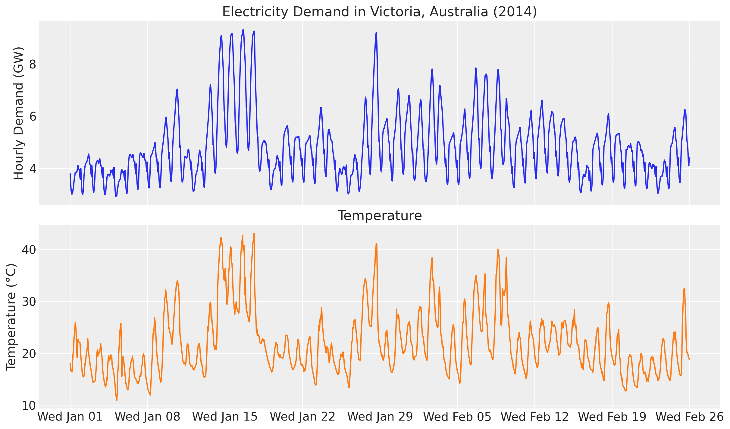
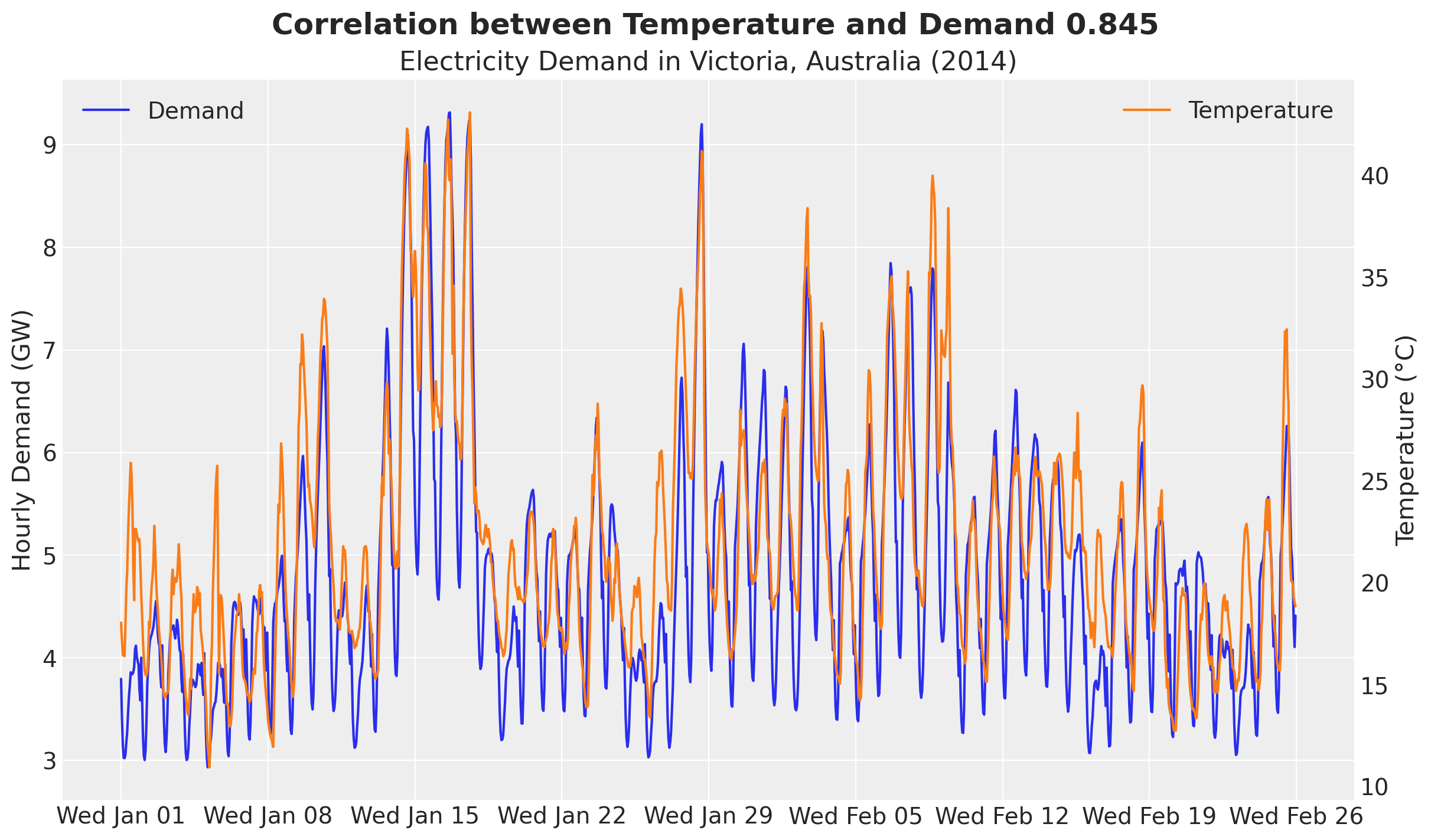
We clearly see an overall positive correlation between temperature and electricity demand. This can be particularly seen when we plot both demand and temperature in the same (twin) axis.
fig, ax = plt.subplots()
ax_twinx = ax.twinx()
ax.plot(demand_dates, demand, c="C0", label="Demand")
ax.set(
    title="Electricity Demand in Victoria, Australia (2014)",
    ylabel="Hourly Demand (GW)",
)
ax_twinx.plot(demand_dates, temperature, c="C1", label="Temperature")
ax_twinx.set(ylabel="Temperature (°C)")
ax.xaxis.set_major_locator(demand_loc)
ax.xaxis.set_major_formatter(demand_fmt)
ax_twinx.grid(None)
ax.legend(loc="upper left")
ax_twinx.legend(loc="upper right")
corr = np.corrcoef(temperature, demand)[0, 1]
fig.suptitle(
    f"Correlation between Temperature and Demand {corr:.3f}",
    fontsize=18,
    fontweight="bold",
);
Besides forecasting, we would also like to understand the relationship between temperature and electricity demand. A good first starting point is to generate a scatter plot of temperature and demand.
fig, ax = plt.subplots()
ax.scatter(temperature, demand)
ax.set(title="Demand vs Temperature", xlabel="Temperature (°C)", ylabel="Demand (GW)");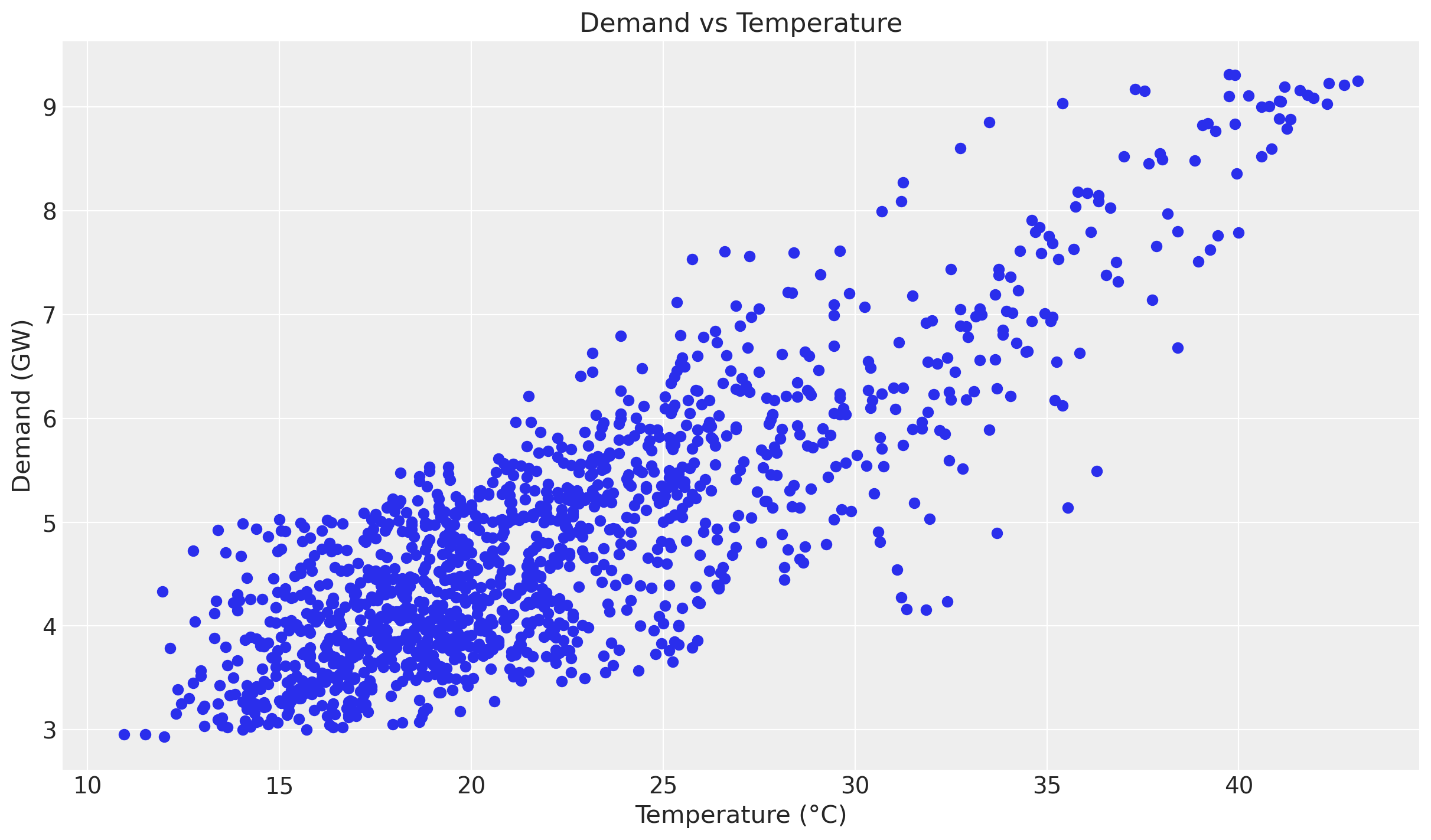
Even though we see a positive relationship between temperature and demand, the relationship is not linear. We can see this by plotting the ratio of demand to temperature.
fig, ax = plt.subplots()
ax.scatter(temperature, demand / temperature, c=demand, cmap="viridis")
cbar = fig.colorbar(ax.collections[0], ax=ax)
cbar.set_label("Demand (GW)")

ax.set(
    title="Demand / Temperature vs Temperature",
    xlabel="Temperature (°C)",
    ylabel="Demand / Temperature",
);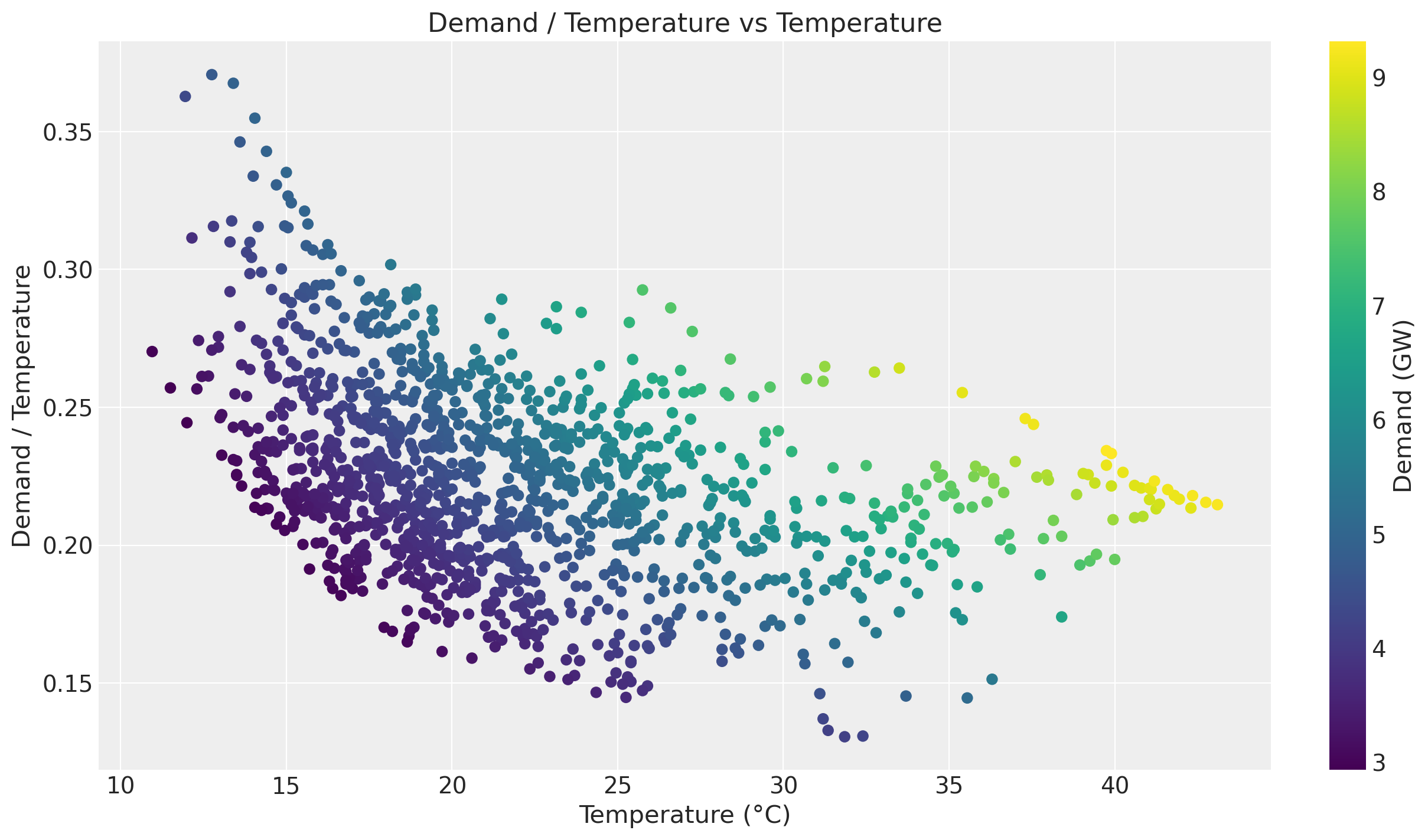
Of course there are strong seasonal effects hidden in these plots. Therefore we want to use a model that can capture thee temperature effect while controlling for other factors.
Training and Test Data
We split the data as in the original example. In addition, we create a day_of_week feature to include in the model later.
num_forecast_steps = 24 * 7 * 2  # Two weeks.
demand_training_data = demand[:-num_forecast_steps]
demand_test_data = demand[-num_forecast_steps:]

temperature_training_data = temperature[:-num_forecast_steps]
temperature_test_data = temperature[-num_forecast_steps:]

demand_dates_training_data = demand_dates[:-num_forecast_steps]
demand_dates_test_data = demand_dates[-num_forecast_steps:]

day_of_week = jnp.array([x.weekday() for x in demand_dates.astype(object)])
day_of_week_training_data = day_of_week[:-num_forecast_steps]
day_of_week_test_data = day_of_week[-num_forecast_steps:]


print(f"Demand training data shape: {demand_training_data.shape}")
print(f"Demand test data shape: {demand_test_data.shape}")
print(f"Temperature training data shape: {temperature_training_data.shape}")
print(f"Temperature test data shape: {temperature_test_data.shape}")
print(f"Day of week training data shape: {day_of_week_training_data.shape}")
print(f"Day of week test data shape: {day_of_week_test_data.shape}")
Demand training data shape: (1008,)
Demand test data shape: (336,)
Temperature training data shape: (1008,)
Temperature test data shape: (336,)
Day of week training data shape: (1008,)
Day of week test data shape: (336,)We can now visualize the training and test data of the demand.
fig, ax = plt.subplots()
ax.plot(demand_dates_training_data, demand_training_data, label="Training Data")
ax.plot(demand_dates_test_data, demand_test_data, label="Test Data")
ax.axvline(
    x=demand_dates_training_data[-1],
    color="black",
    linestyle="--",
    label="Training-Test Split",
)
ax.set(title="Demand Data", ylabel="Demand (GW)")
ax.legend()
ax.xaxis.set_major_locator(demand_loc)
ax.xaxis.set_major_formatter(demand_fmt);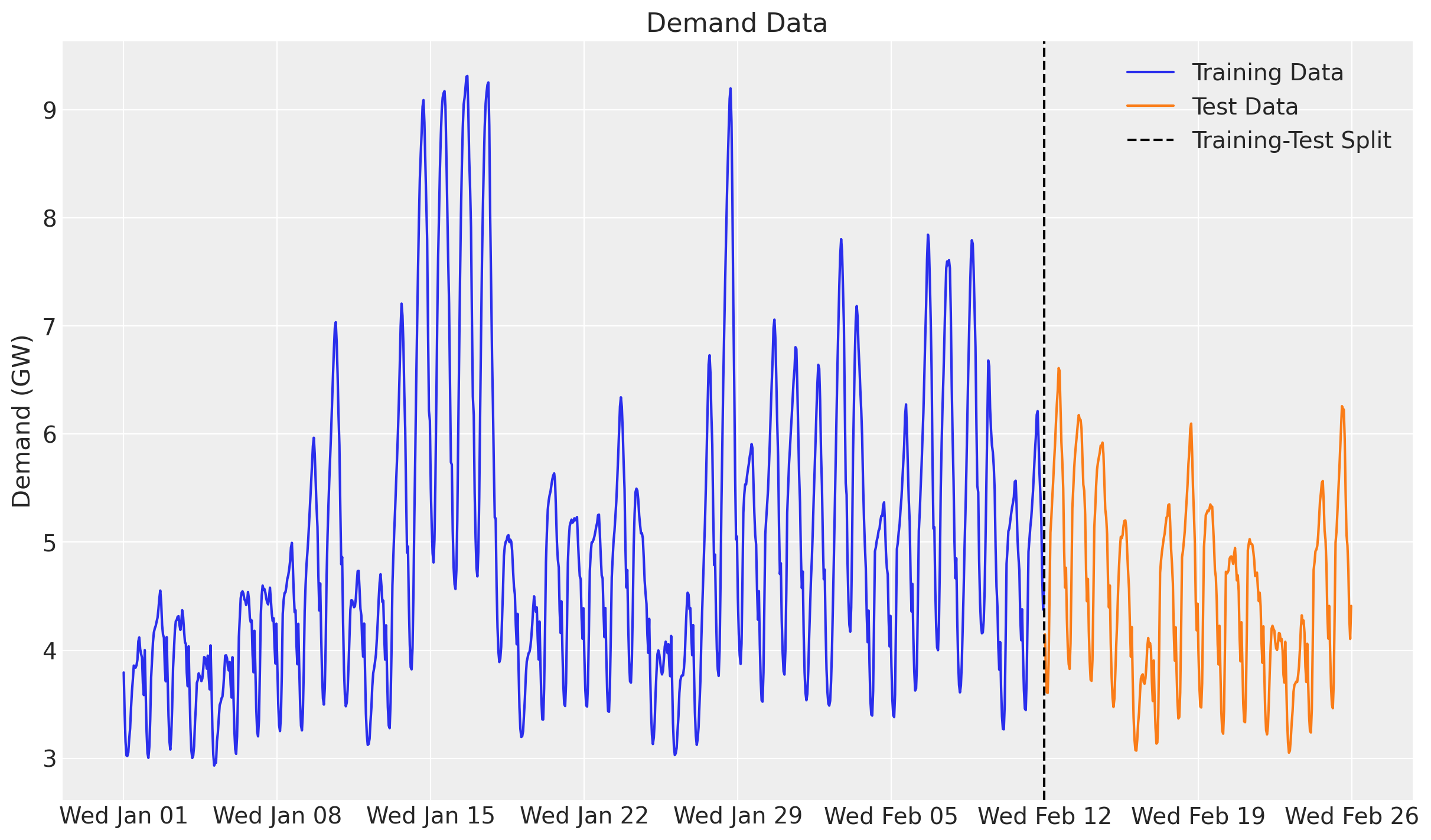
Model Specification
Here is a description of the modeling strategy:
- We use a linear model to predict demand as a function of temperature and two seasonal effects: hour of day and day of week. We use Zero-Sum Normal distributions to model these seasonal effects.
- We use a Matérn 5/2 kernel to model the temperature effect on demand using the Hilbert Space Gaussian Process (HSGP) approximation from NumPyro (see here).
- The noise scale will vary with the temperature.
- We use a Student-t distribution to model the residual error.
GP Prior Parameters
One key component of specifying Gaussian processes is to set the length scale and amplitude parameters. Se use an optimization strategy to set these parameters by assuming they both come from an Inverse-Gamma distribution, while specifying the support.
# For the amplitude, we set the values inspired on the range of the demand / temperature
# ratio above.
amplitude_params, ax = pz.maxent(pz.InverseGamma(), lower=0.1, upper=0.5)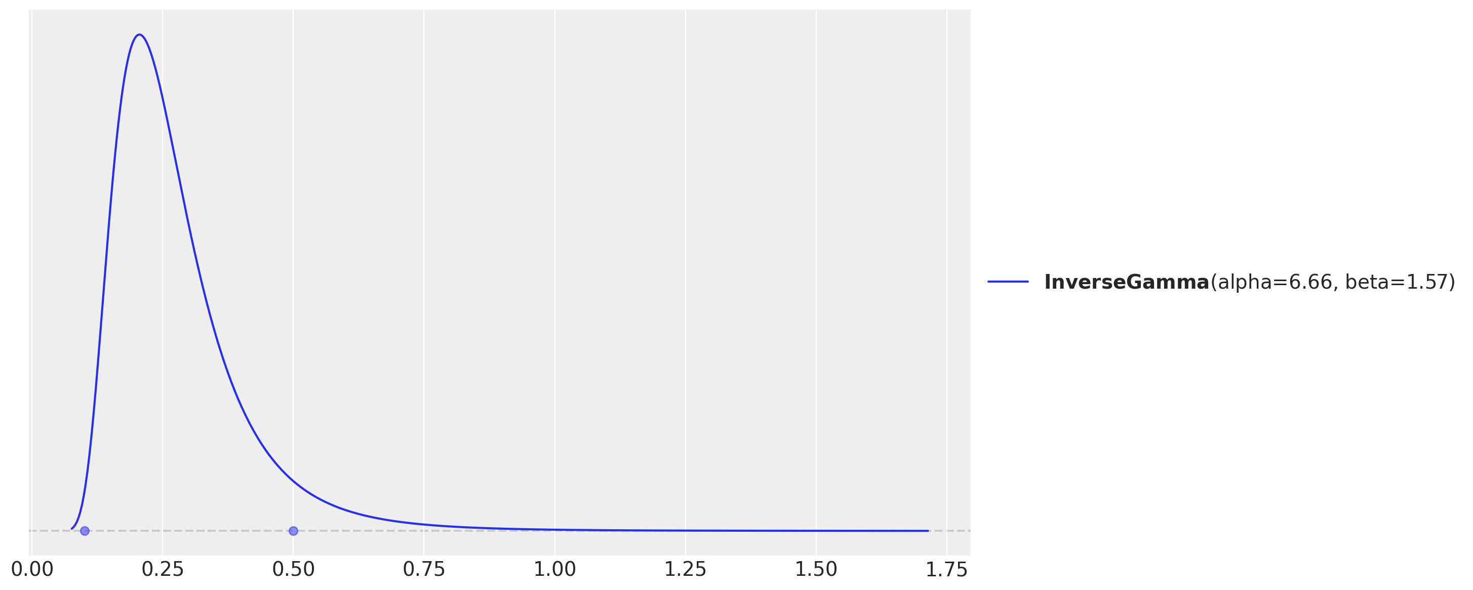
# As we want to use the GP to model the temperature effect, we need to set the length
# scale parameter.
# We are expecting these effects to be seen at the order of units or tens of units,
# so we expect the length scale to be between 3 and 10.
length_scale_params, ax = pz.maxent(pz.InverseGamma(), lower=3, upper=10)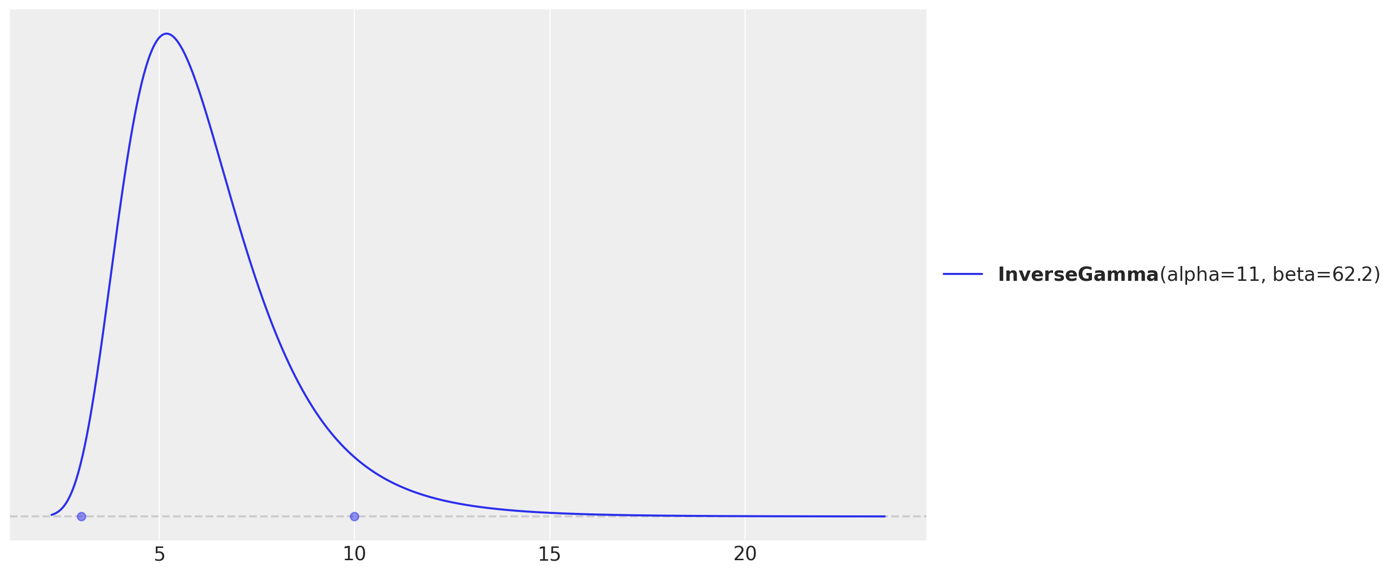
Periodic Features
For the hour of day effect, we use the repeating trick explained in the example From Pyro to NumPyro: Forecasting Hierarchical Models - Part I.
def periodic_repeat_jax(tensor: Array, size: int, dim: int) -> Array:
    """
    Repeat a period-sized tensor up to given size using JAX.

    Parameters
    ----------
    tensor : Array
        A JAX array to be repeated.
    size : int
        Desired size of the result along dimension `dim`.
    dim : int
        The tensor dimension along which to repeat.

    Returns
    -------
    Array
        The repeated tensor.

    References
    ----------
    Thttps://docs.pyro.ai/en/stable/ops.html#pyro.ops.tensor_utils.periodic_repeat
    """
    assert isinstance(size, int) and size >= 0
    assert isinstance(dim, int)
    if dim >= 0:
        dim -= tensor.ndim

    period = tensor.shape[dim]
    repeats = [1] * tensor.ndim
    repeats[dim] = (size + period - 1) // period
    result = jnp.tile(tensor, repeats)

    slices = [slice(None)] * tensor.ndim
    slices[dim] = slice(None, size)

    return result[tuple(slices)]
Now we are ready to specify the NumPyro model.
def model(
    temperature: Float[Array, " t"],
    day_of_week: Int[Array, " t"],
    ell: float = 55.0,
    m: int = 25,
    demand: Float[Array, " t"] | None = None,
) -> None:
    t_max = temperature.size

    # Intercept
    intercept = numpyro.sample("intercept", dist.Normal(loc=0, scale=2))

    # GP Parameters
    ## Amplitude
    alpha = numpyro.sample("alpha", dist.InverseGamma(concentration=6.66, rate=1.57))
    ## Length Scale
    length_scale = numpyro.sample(
        "length_scale", dist.InverseGamma(concentration=11, rate=62.2)
    )
    ## Scale Factor
    scale_factor = numpyro.sample("scale", dist.HalfNormal(scale=0.5))
    ## Noise Scale
    # Degrees of Freedom for the Student-t distribution
    nu = numpyro.sample("nu", dist.Gamma(concentration=8, rate=3))

    # Temperature Effect as a HSGP
    beta_temperature = numpyro.deterministic(
        "beta_temperature",
        hsgp_matern(
            x=temperature,
            nu=5 / 2,
            alpha=alpha,
            length=length_scale,
            ell=ell,
            m=m,
        ),
    )

    # Hour of Day Effect
    scale_hour_of_day = numpyro.sample("scale_hour_of_day", dist.HalfNormal(scale=0.5))
    hour_of_day_effect = numpyro.sample(
        "hour_of_day_effect",
        dist.ZeroSumNormal(scale=scale_hour_of_day, event_shape=(24,)),
    )
    hour_of_day_effect_repeat = periodic_repeat_jax(hour_of_day_effect, t_max, dim=0)

    # Day of Week Effect
    scale_day_of_week = numpyro.sample("scale_day_of_week", dist.HalfNormal(scale=0.5))
    day_of_week_effect = numpyro.sample(
        "day_of_week_effect",
        dist.ZeroSumNormal(scale=scale_day_of_week, event_shape=(7,)),
    )

    # Expected Value
    mu = (
        intercept
        + beta_temperature * temperature
        + hour_of_day_effect_repeat
        + day_of_week_effect[day_of_week]
    )

    scale = scale_factor * jnp.sqrt(temperature)

    # Likelihood
    with numpyro.plate("data", t_max):
        numpyro.sample("obs", dist.StudentT(df=nu, loc=mu, scale=scale), obs=demand)
Let’s visualize the models structure.
numpyro.render_model(
    model=model,
    model_kwargs={
        "temperature": temperature_training_data,
        "day_of_week": day_of_week_training_data,
        "demand": demand_training_data,
    },
    render_distributions=True,
    render_params=True,
)
Prior Predictive Checks
Before we fit the model, let’s visualize the prior predictive distribution.
prior_predictive = Predictive(model=model, num_samples=2_000, return_sites=["obs"])

rng_key, rng_subkey = random.split(rng_key)
prior_predictive_sampels = prior_predictive(
    rng_subkey,
    temperature=temperature_training_data,
    day_of_week=day_of_week_training_data,
)

idata_prior = az.from_dict(
    prior_predictive={k: v[None, ...] for k, v in prior_predictive_sampels.items()},
    coords={"time": demand_dates_training_data},
    dims={"obs": ["time"]},
)
fig, ax = plt.subplots()
az.plot_hdi(
demand_dates_training_data,
idata_prior["prior_predictive"]["obs"],
hdi_prob=0.94,
smooth=False,
color="C0",
fill_kwargs={"alpha": 0.3, "label": "94% HDI"},
ax=ax,
)
az.plot_hdi(
demand_dates_training_data,
idata_prior["prior_predictive"]["obs"],
smooth=False,
hdi_prob=0.5,
color="C0",
fill_kwargs={"alpha": 0.5, "label": "50% HDI"},
ax=ax,
)
ax.plot(
demand_dates_training_data, demand_training_data, c="black", label="Training Data"
)
ax.legend()
ax.set(title="Prior Predictive Checks", ylabel="Demand (GW)", xlabel="Time")
ax.xaxis.set_major_locator(demand_loc)
ax.xaxis.set_major_formatter(demand_fmt);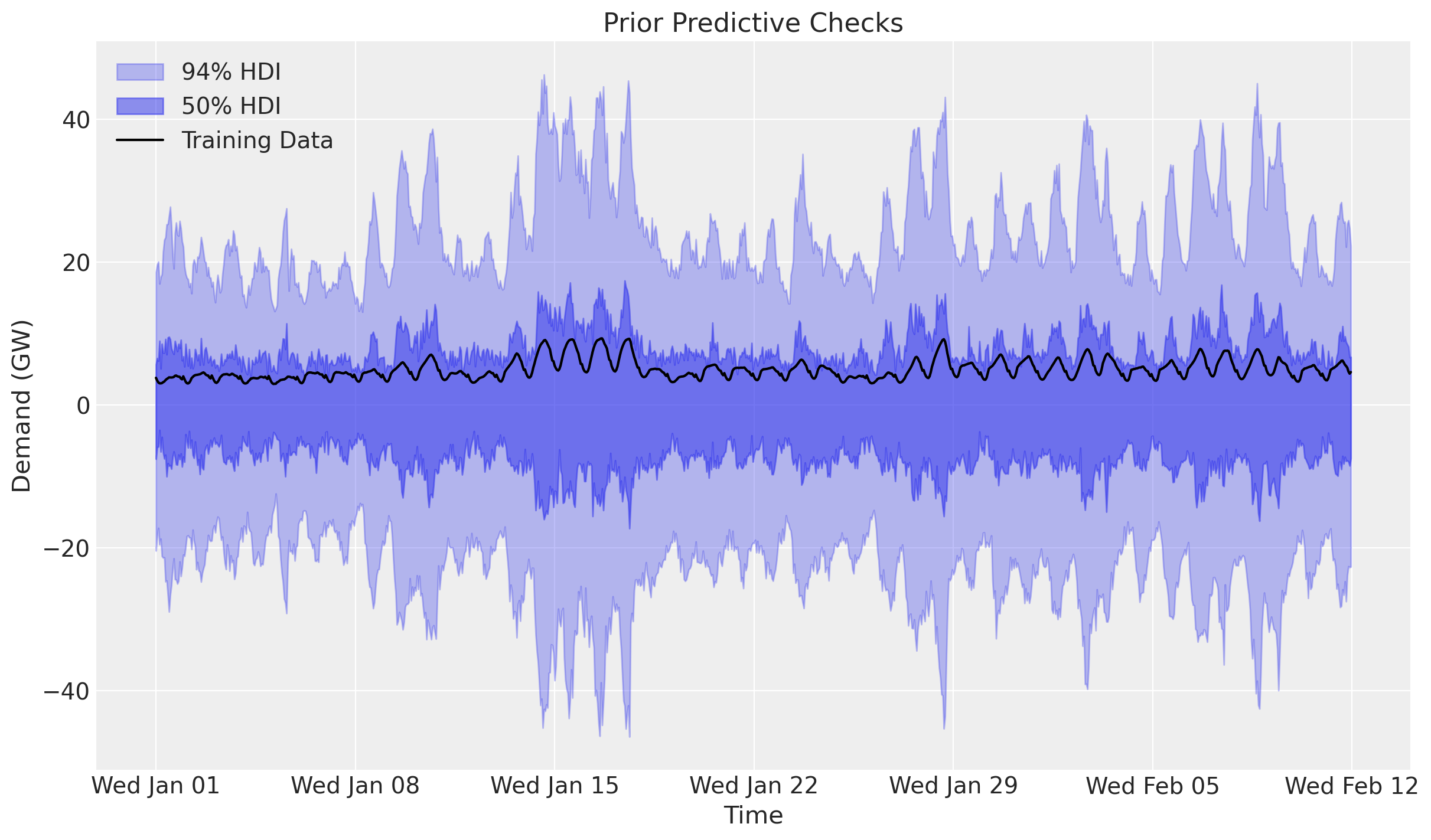
The prior predictive distribution is not too far from the training data but is not very restrictive either.
Inference with SVI
We use stochastic variational inference to fit the model.
guide = AutoNormal(model)
optimizer = numpyro.optim.Adam(step_size=0.005)
svi = SVI(model, guide, optimizer, loss=Trace_ELBO())
num_steps = 50_000

rng_key, rng_subkey = random.split(key=rng_key)

svi_result = svi.run(
    rng_subkey,
    num_steps,
    temperature=temperature_training_data,
    day_of_week=day_of_week_training_data,
    demand=demand_training_data,
)

fig, ax = plt.subplots(figsize=(9, 6))
ax.plot(svi_result.losses)
ax.set_yscale("log")
ax.set_title("ELBO loss", fontsize=18, fontweight="bold");
100%|██████████| 50000/50000 [00:15<00:00, 3246.70it/s, init loss: 6238.8652, avg. loss [47501-50000]: 825.7322]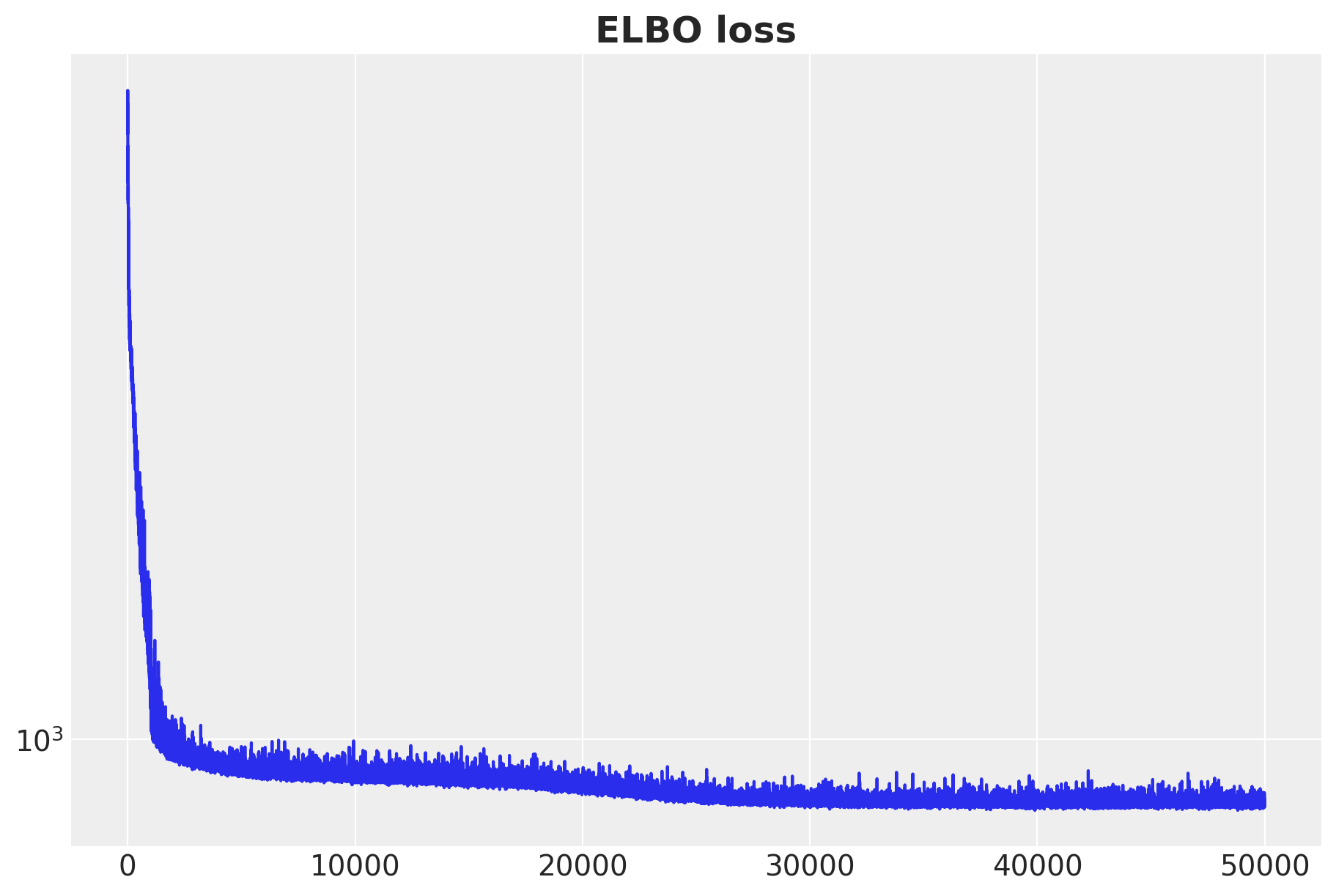
The ELBO loss is decreasing as expected.
Posterior Predictive Checks
We now generate samples for the training and test data. We are interested in both the likelihood (demand) and the posterior distribution of the temperature effect.
posterior = Predictive(
    model=model,
    guide=guide,
    params=svi_result.params,
    num_samples=5_000,
    return_sites=["beta_temperature", "obs"],
)

rng_key, rng_subkey = random.split(rng_key)
train_posterior_samples = posterior(
    rng_subkey,
    temperature=temperature_training_data,
    day_of_week=day_of_week_training_data,
)

rng_key, rng_subkey = random.split(rng_key)
test_posterior_samples = posterior(
    rng_subkey, temperature=temperature, day_of_week=day_of_week
)
idata_train = az.from_dict(
posterior={k: v[None, ...] for k, v in train_posterior_samples.items()},
coords={"time": demand_dates_training_data},
dims={"obs": ["time"], "beta_temperature": ["time"]},
)
idata_test = az.from_dict(
posterior={k: v[None, ...] for k, v in test_posterior_samples.items()},
coords={"time": demand_dates},
dims={"obs": ["time"], "beta_temperature": ["time"]},
)Forecast
We evaluate the forecast using the Continuous Ranked Probability Score (CRPS).
@jax.jit
def crps(
    truth: Float[Array, " t"],
    pred: Float[Array, "n_samples t"],
    sample_weight: Float[Array, " t"] | None = None,
) -> Float[Array, ""]:
    if pred.shape[1:] != (1,) * (pred.ndim - truth.ndim - 1) + truth.shape:
        raise ValueError(
            f"""Expected pred to have one extra sample dim on left.
            Actual shapes: {pred.shape} versus {truth.shape}"""
        )

    absolute_error = jnp.mean(jnp.abs(pred - truth), axis=0)

    num_samples = pred.shape[0]
    if num_samples == 1:
        return jnp.average(absolute_error, weights=sample_weight)

    pred = jnp.sort(pred, axis=0)
    diff = pred[1:] - pred[:-1]
    weight = jnp.arange(1, num_samples) * jnp.arange(num_samples - 1, 0, -1)
    weight = weight.reshape(weight.shape + (1,) * (diff.ndim - 1))

    per_obs_crps = absolute_error - jnp.sum(diff * weight, axis=0) / num_samples**2
    return jnp.average(per_obs_crps, weights=sample_weight)


crps_train = crps(
    demand_training_data, jnp.array(idata_train["posterior"]["obs"].sel(chain=0))
)

crps_test = crps(
    demand_test_data,
    jnp.array(
        idata_test["posterior"]["obs"]
        .sel(chain=0)
        .isel(time=slice(demand_dates_training_data.size, None))
    ),
)
We can now compare the posterior predictive distribution with the training and test data.
fig, ax = plt.subplots()

az.plot_hdi(
    demand_dates_training_data,
    idata_train["posterior"]["obs"],
    hdi_prob=0.94,
    smooth=False,
    color="C0",
    fill_kwargs={"alpha": 0.2, "label": "94% HDI"},
    ax=ax,
)

az.plot_hdi(
    demand_dates_training_data,
    idata_train["posterior"]["obs"],
    hdi_prob=0.5,
    smooth=False,
    color="C0",
    fill_kwargs={"alpha": 0.4, "label": "50% HDI"},
    ax=ax,
)

ax.plot(
    demand_dates_training_data,
    idata_train["posterior"]["obs"].mean(dim=("chain", "draw")),
    c="C0",
    label="Posterior Mean",
)

az.plot_hdi(
    demand_dates_test_data,
    idata_test["posterior"]["obs"].isel(
        time=slice(demand_dates_training_data.size, None)
    ),
    hdi_prob=0.94,
    smooth=False,
    color="C1",
    fill_kwargs={"alpha": 0.2, "label": "94% HDI"},
    ax=ax,
)

az.plot_hdi(
    demand_dates_test_data,
    idata_test["posterior"]["obs"].isel(
        time=slice(demand_dates_training_data.size, None)
    ),
    hdi_prob=0.5,
    smooth=False,
    color="C1",
    fill_kwargs={"alpha": 0.4, "label": "50% HDI"},
    ax=ax,
)

ax.plot(
    demand_dates_test_data,
    idata_test["posterior"]["obs"]
    .isel(time=slice(demand_dates_training_data.size, None))
    .mean(dim=("chain", "draw")),
    c="C1",
    label="Posterior Mean",
)

ax.plot(
    demand_dates_training_data, demand_training_data, c="black", label="Training Data"
)

ax.plot(demand_dates_test_data, demand_test_data, c="black", label="Test Data")

ax.legend(loc="upper center", bbox_to_anchor=(0.5, -0.1), ncol=4)
ax.set(
    title=f"Train CRPS: {crps_train:.3f}, Test CRPS: {crps_test:.3f}",
    ylabel="Demand (GW)",
    xlabel="Time",
)
ax.xaxis.set_major_locator(demand_loc)
ax.xaxis.set_major_formatter(demand_fmt)

fig.suptitle("Posterior Predictive Checks", fontsize=18, fontweight="bold");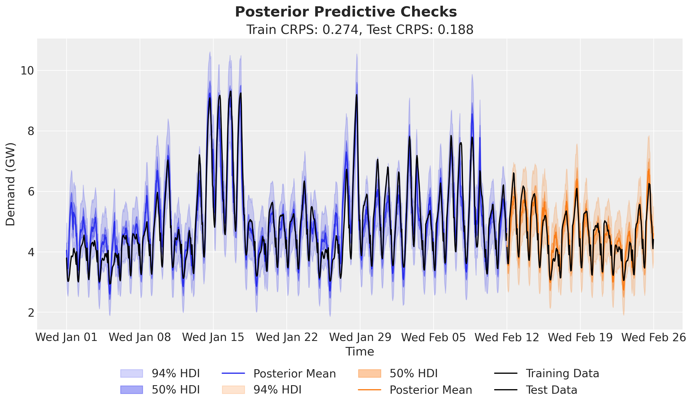
The predictions look very good! They are actually look much better that the basic linear model used in the TensorFlow Probability tutorial (which is fine as they are focusing on the core API description).
Temperature Effect on Demand
Being happy about the forecast performance, we can dig deeper into the temperature effect. First we simply plot the predictions and the raw values.
fig, ax = plt.subplots()

az.plot_hdi(
    temperature_training_data,
    idata_train["posterior"]["obs"],
    hdi_prob=0.94,
    smooth=True,
    color="C0",
    fill_kwargs={"alpha": 0.3, "label": "94% HDI"},
    ax=ax,
)

az.plot_hdi(
    temperature_training_data,
    idata_train["posterior"]["obs"],
    hdi_prob=0.5,
    smooth=True,
    color="C0",
    fill_kwargs={"alpha": 0.5, "label": "50% HDI"},
    ax=ax,
)

ax.scatter(temperature_training_data, demand_training_data, c="black")
ax.set(title="Demand vs Temperature", xlabel="Temperature (°C)", ylabel="Demand (GW)");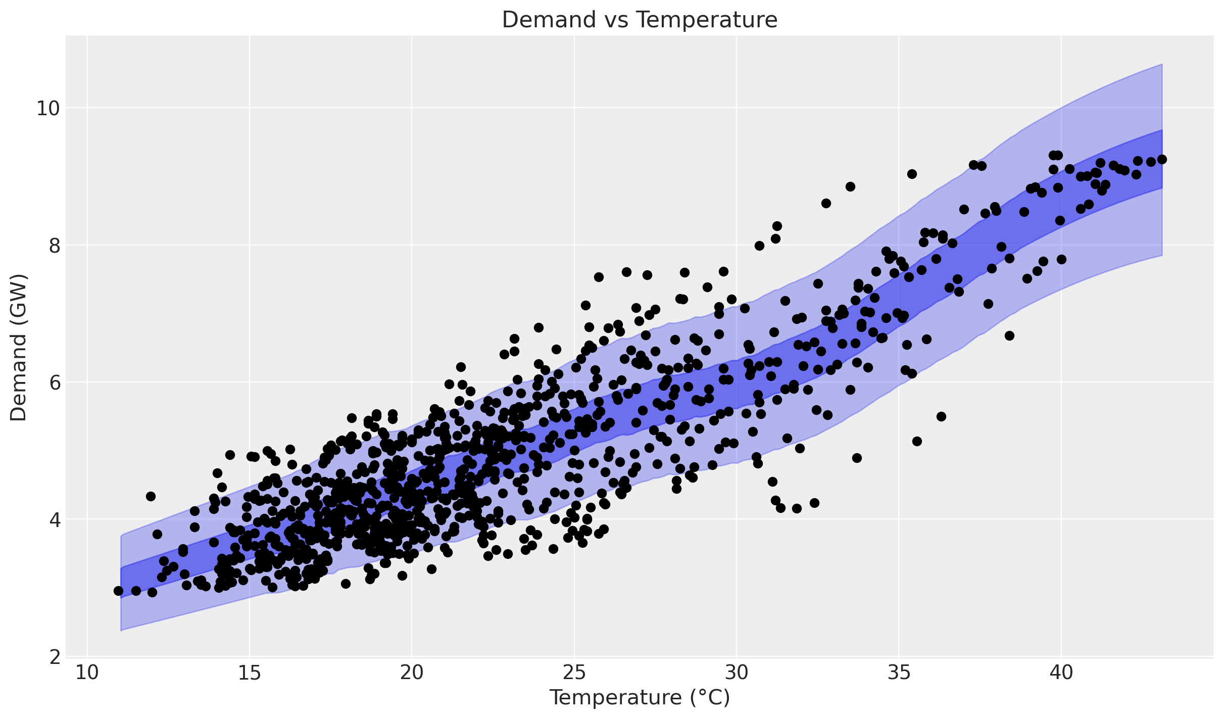
The non-linearity is clearly visible! Nevertheless, we are interested in the laten unseen variable between temperature and demand. In therms of the model, we are interested in the posterior distribution of the Gaussian Process component.
fig, ax = plt.subplots()

az.plot_hdi(
    temperature_training_data,
    idata_train["posterior"]["beta_temperature"],
    hdi_prob=0.94,
    smooth=True,
    color="C1",
    fill_kwargs={"alpha": 0.3, "label": "94% HDI"},
    ax=ax,
)

az.plot_hdi(
    temperature_training_data,
    idata_train["posterior"]["beta_temperature"],
    hdi_prob=0.5,
    smooth=True,
    color="C1",
    fill_kwargs={"alpha": 0.5, "label": "50% HDI"},
    ax=ax,
)

ax.set(
    title="Temperature Effect on Demand",
    xlabel="Temperature (°C)",
    ylabel="Effect on Demand",
);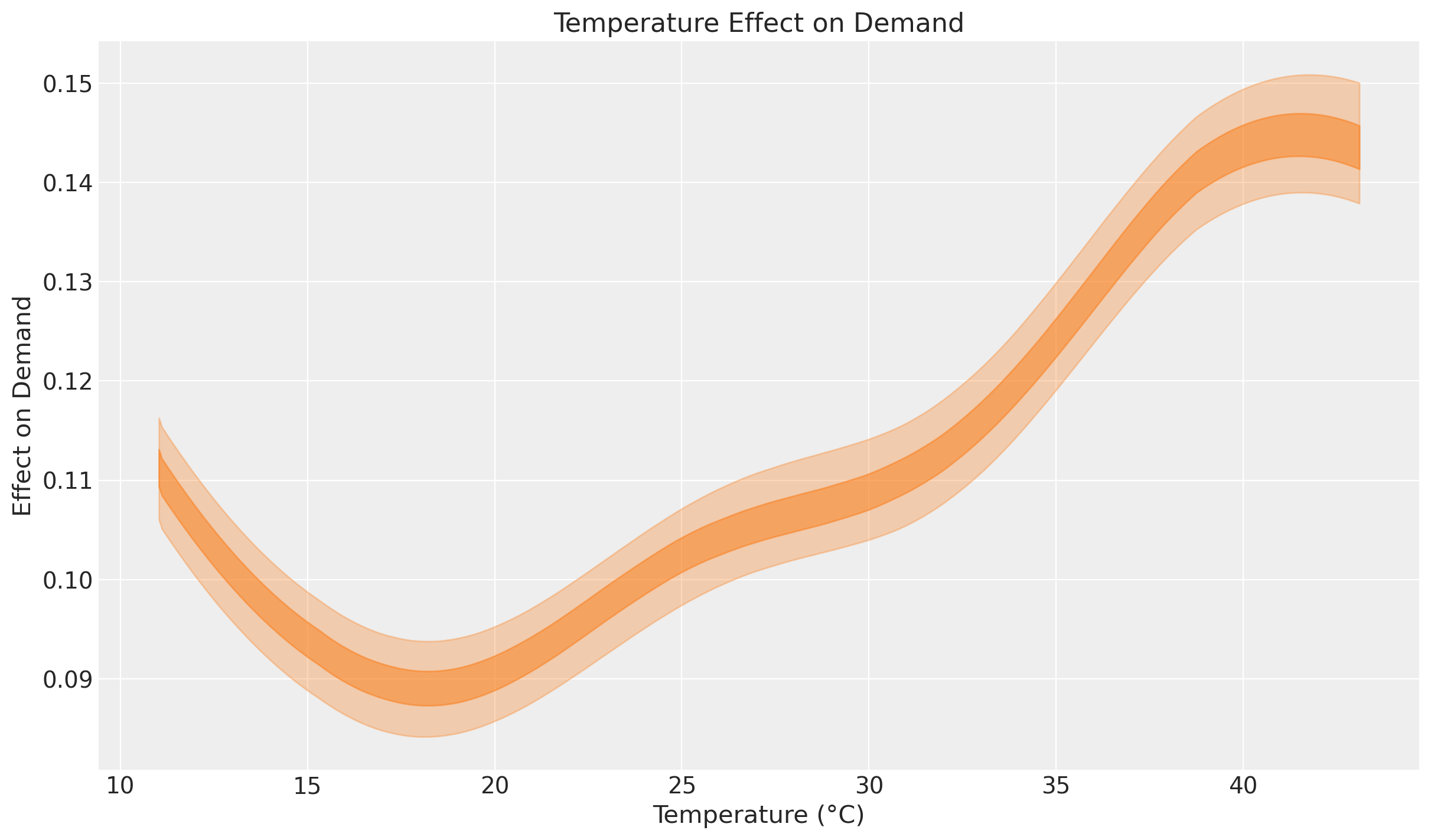
This effect plot coincided with the comment on the exploratory data analysis https://otexts.com/fpp2/scatterplots.html by Hyndman and Athanasopoulos.
“It is clear that high demand occurs when temperatures are high due to the effect of air-conditioning. But there is also a heating effect, where demand increases for very low temperatures.”
Indeed, we see that at the extremes of the common temperature range, the temperature effect on demand increases! Heating and cooling usually happens outside the range \(15\)°C - \(25\)°C.