In this post I present a concrete case study illustrating some techniques to improve model performance in class-imbalanced classification problems. The methodologies described here are based on Chapter 16: Remedies for Severe Class Imbalance of the (great!) book Applied Predictive Modeling by Max Kuhn and Kjell Johnson. I absolutely recommend this reference to anyone interested in predictive modeling.

This notebook should serve as an extension of my talk given at satRday Berlin 2019: A conference for R users in Berlin. Here are the slides:

You can download the final model_list object containing the trained models and functions here.

The Data Set

The data set we are going to work with is the one suggested in Exercise 16.1 of the reference mentioned above:

The “adult” data set at the UCI Machine Learning Repository is derived from census records. In these data, the goal is to predict whether a person’s income was large (defined in 1994 as more than $50K) or small. The predictors include educational level, type of job (e.g., never worked, and local government), capital gains/losses, work hours per week, native country, and so on.

The data are contained in the arules package.

Remark The objective of this post is not to find the “best” predictive model, but rather explore the techniques to handle class imbalance. There is a large amount of literature around this concrete data set, e.g. see this post or the Kaggle kernels.

Prepare Notebook

# Load Libraries
library(caret)
library(gbm)
library(magrittr)
library(pROC)
library(tidyverse)

# Allow parallel computation.
library(parallel)
library(doParallel)

# Load Data
data(AdultUCI, package = "arules")
raw_data <- AdultUCI

Data Audit

Let us start with first exploration of the data set:

# See Data Structure. 
glimpse(raw_data)

## Observations: 48,842
## Variables: 15
## $ age              <int> 39, 50, 38, 53, 28, 37, 49, 52, 31, 42, 37, 30,…
## $ workclass        <fct> State-gov, Self-emp-not-inc, Private, Private, …
## $ fnlwgt           <int> 77516, 83311, 215646, 234721, 338409, 284582, 1…
## $ education        <ord> Bachelors, Bachelors, HS-grad, 11th, Bachelors,…
## $ `education-num`  <int> 13, 13, 9, 7, 13, 14, 5, 9, 14, 13, 10, 13, 13,…
## $ `marital-status` <fct> Never-married, Married-civ-spouse, Divorced, Ma…
## $ occupation       <fct> Adm-clerical, Exec-managerial, Handlers-cleaner…
## $ relationship     <fct> Not-in-family, Husband, Not-in-family, Husband,…
## $ race             <fct> White, White, White, Black, Black, White, Black…
## $ sex              <fct> Male, Male, Male, Male, Female, Female, Female,…
## $ `capital-gain`   <int> 2174, 0, 0, 0, 0, 0, 0, 0, 14084, 5178, 0, 0, 0…
## $ `capital-loss`   <int> 0, 0, 0, 0, 0, 0, 0, 0, 0, 0, 0, 0, 0, 0, 0, 0,…
## $ `hours-per-week` <int> 40, 13, 40, 40, 40, 40, 16, 45, 50, 40, 80, 40,…
## $ `native-country` <fct> United-States, United-States, United-States, Un…
## $ income           <ord> small, small, small, small, small, small, small…

The variable we are interested to predict is income. Let us see its distribution.

raw_data %>% 
  count(income) %>% 
  mutate(share = n / sum(n))

## # A tibble: 3 x 3
##   income     n share
##   <ord>  <int> <dbl>
## 1 small  24720 0.506
## 2 large   7841 0.161
## 3 <NA>   16281 0.333

The first thing we see is that 1/3 of the data has no income label.

In addition, as described in the arules package’s documentation, the fnlwgt (final weight) and education can be removed from the data. The last one being another representation of the attribute education-num. To see this

raw_data %>% 
  select(education, `education-num`) %>% 
  table()

##               education-num
## education          1     2     3     4     5     6     7     8     9    10
##   Preschool       83     0     0     0     0     0     0     0     0     0
##   1st-4th          0   247     0     0     0     0     0     0     0     0
##   5th-6th          0     0   509     0     0     0     0     0     0     0
##   7th-8th          0     0     0   955     0     0     0     0     0     0
##   9th              0     0     0     0   756     0     0     0     0     0
##   10th             0     0     0     0     0  1389     0     0     0     0
##   11th             0     0     0     0     0     0  1812     0     0     0
##   12th             0     0     0     0     0     0     0   657     0     0
##   HS-grad          0     0     0     0     0     0     0     0 15784     0
##   Prof-school      0     0     0     0     0     0     0     0     0     0
##   Assoc-acdm       0     0     0     0     0     0     0     0     0     0
##   Assoc-voc        0     0     0     0     0     0     0     0     0     0
##   Some-college     0     0     0     0     0     0     0     0     0 10878
##   Bachelors        0     0     0     0     0     0     0     0     0     0
##   Masters          0     0     0     0     0     0     0     0     0     0
##   Doctorate        0     0     0     0     0     0     0     0     0     0
##               education-num
## education         11    12    13    14    15    16
##   Preschool        0     0     0     0     0     0
##   1st-4th          0     0     0     0     0     0
##   5th-6th          0     0     0     0     0     0
##   7th-8th          0     0     0     0     0     0
##   9th              0     0     0     0     0     0
##   10th             0     0     0     0     0     0
##   11th             0     0     0     0     0     0
##   12th             0     0     0     0     0     0
##   HS-grad          0     0     0     0     0     0
##   Prof-school      0     0     0     0   834     0
##   Assoc-acdm       0  1601     0     0     0     0
##   Assoc-voc     2061     0     0     0     0     0
##   Some-college     0     0     0     0     0     0
##   Bachelors        0     0  8025     0     0     0
##   Masters          0     0     0  2657     0     0
##   Doctorate        0     0     0     0     0   594

In addition, let us see the distribution (share) of the variable country:

raw_data %>% 
  count(`native-country`) %>%
  mutate(n = n / sum(n)) %>% 
  mutate(`native-country` = reorder(`native-country` , n)) %>% 
  ggplot(mapping = aes(x = `native-country`, y = n)) +
    geom_bar(stat = "identity", color = "black") + 
    coord_flip() +
    labs(title = "Country Distribution", x = "", y = "")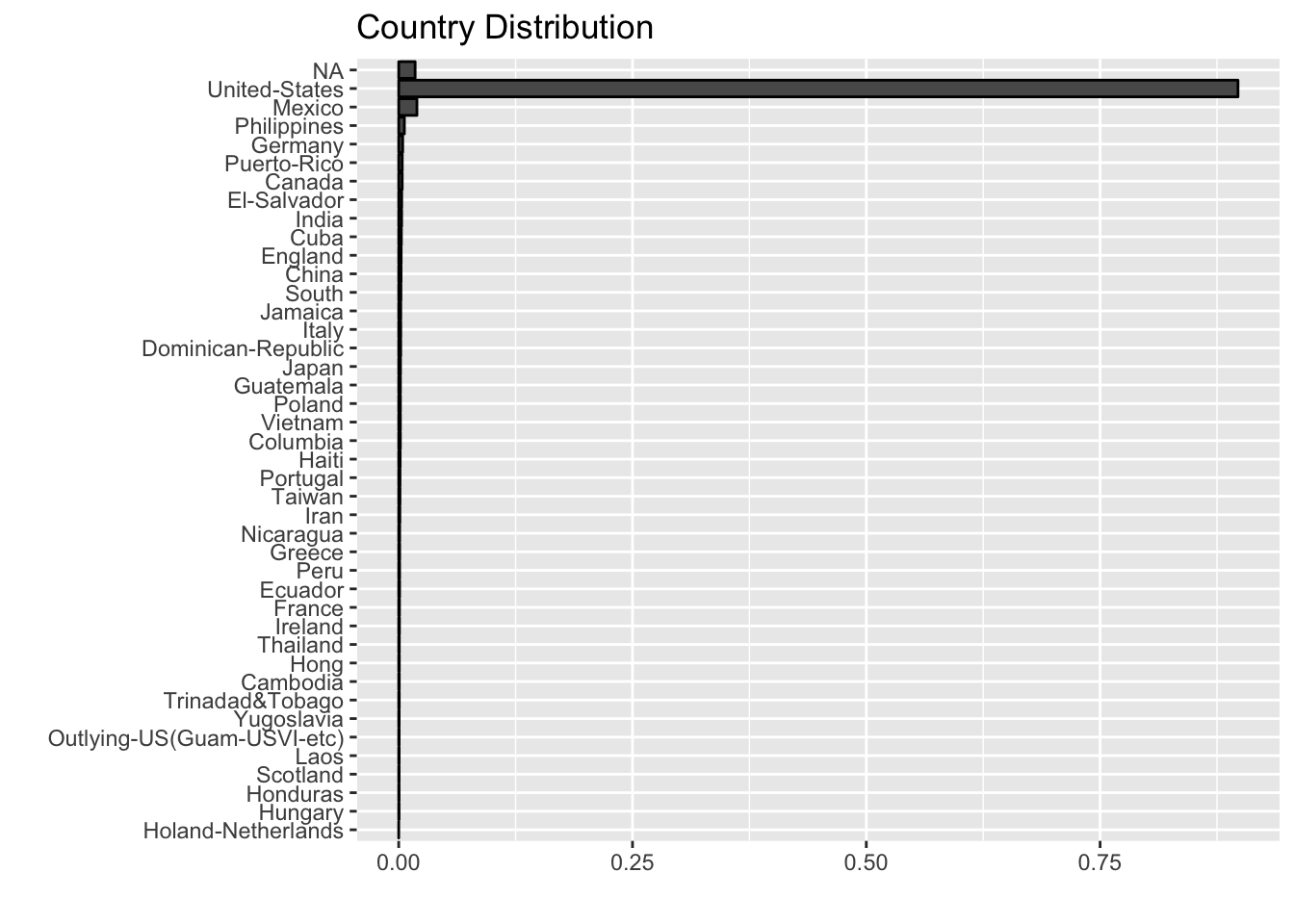

Most of the samples come from the United States. In a first iteration, we are going to omit this variable as well.

We therefore consider the filtered data set:

format_raw_data <- function(df) {
  
  output_df_df <- df %>% 
   filter(!is.na(income)) %>% 
   select(- fnlwgt, - education, - `native-country`)
  
  return(output_df_df)
}

data_df <- format_raw_data(df = raw_data)

Remark: We could have done a deeper analysis on the NA values for the variable income, but we just drop them for simplicity.

We are going to store function, models and other parameters in a list (to be able to user later).

# Define storing list. 
model_list <- vector(mode = "list")

model_list[["functions"]] <- list(format_raw_data = format_raw_data)

Exploratory Data Analysis

Dependent Variable

Let us see the distribution of the income variable.

data_df %>% 
  count(income) %>% 
  mutate(n = n / sum(n))

## # A tibble: 2 x 2
##   income     n
##   <ord>  <dbl>
## 1 small  0.759
## 2 large  0.241

data_df %>% 
  count(income) %>% 
  ggplot(mapping = aes(x = income, y = n, fill = income)) +
  geom_bar(stat = "identity", color = "black") +
  labs(title = "Income Distribution", y = "") +
  scale_fill_brewer(palette = "Set1")

That is, the income variable is not balanced.

Independent Variables

Next we explore each predictor variable.

data_df %>% 
  ggplot(mapping = aes(x = age, y = ..density.., fill = income)) +
  geom_density(alpha = 0.8) +
  labs(title = "Age Distribution") +
  scale_fill_brewer(palette = "Set1")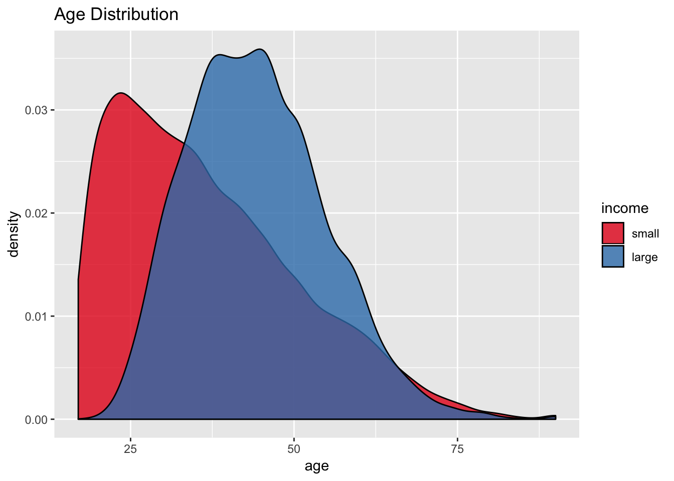

data_df %>% 
  ggplot(mapping = aes(x = income, y = age, fill = income)) +
  geom_boxplot() +
  labs(title = "Age Distribution") +
  scale_fill_brewer(palette = "Set1")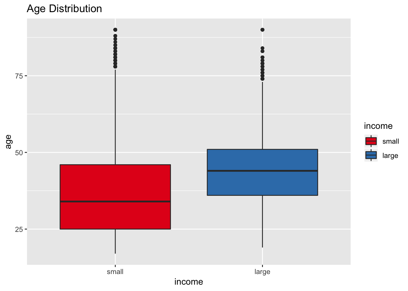

It seems that the age attribute could potentially be a good predictor for income.

Workclass

Many of the features are categorical variables, therefore we write generic functions to generate the plots.

get_bar_plot <- function (df, var_name, sort_cols = TRUE) {
  
  var_name_sym <- rlang::sym(var_name)
  
  count_df <- df %>% count(!!var_name_sym ) 
  
  if (sort_cols) {
    count_df %<>% mutate(!!var_name_sym  := reorder(!!var_name_sym , n))
  }
     
  count_df %>% 
    ggplot(mapping = aes(x = !!var_name_sym , y = n)) +
    geom_bar(stat = "identity", fill = "purple4") + 
    coord_flip() +
    labs(title = var_name) + scale_fill_brewer(palette = "Set1")
    
}

get_bar_plot(df = data_df, var_name = "workclass")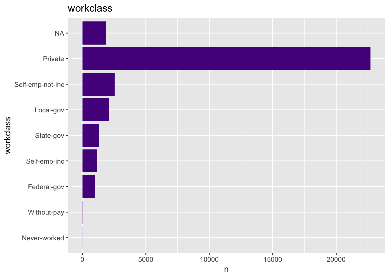

get_split_bar_plot <- function(df, var_name, group_var_name, sort_cols = TRUE) {
  
  var_name_sym <- rlang::sym(var_name)
  group_var_name_sym <- rlang::sym(group_var_name)
  
  count_df <- df %>% count(!!var_name_sym, !!group_var_name_sym) 
  
  if (sort_cols) {
    count_df %<>% mutate(!!var_name_sym  := reorder(!!var_name_sym , n))
  }
  
  count_df %>% 
    ggplot(mapping = aes(x = !!var_name_sym, y = n, fill = !!group_var_name_sym)) +
    geom_bar(stat = "identity", color = "black") + 
    coord_flip() +
    labs(title = var_name) +
    facet_grid(cols = vars(!!group_var_name_sym)) +
    scale_fill_brewer(palette = "Set1")
}

get_split_bar_plot(df = data_df, var_name = "workclass", group_var_name = "income")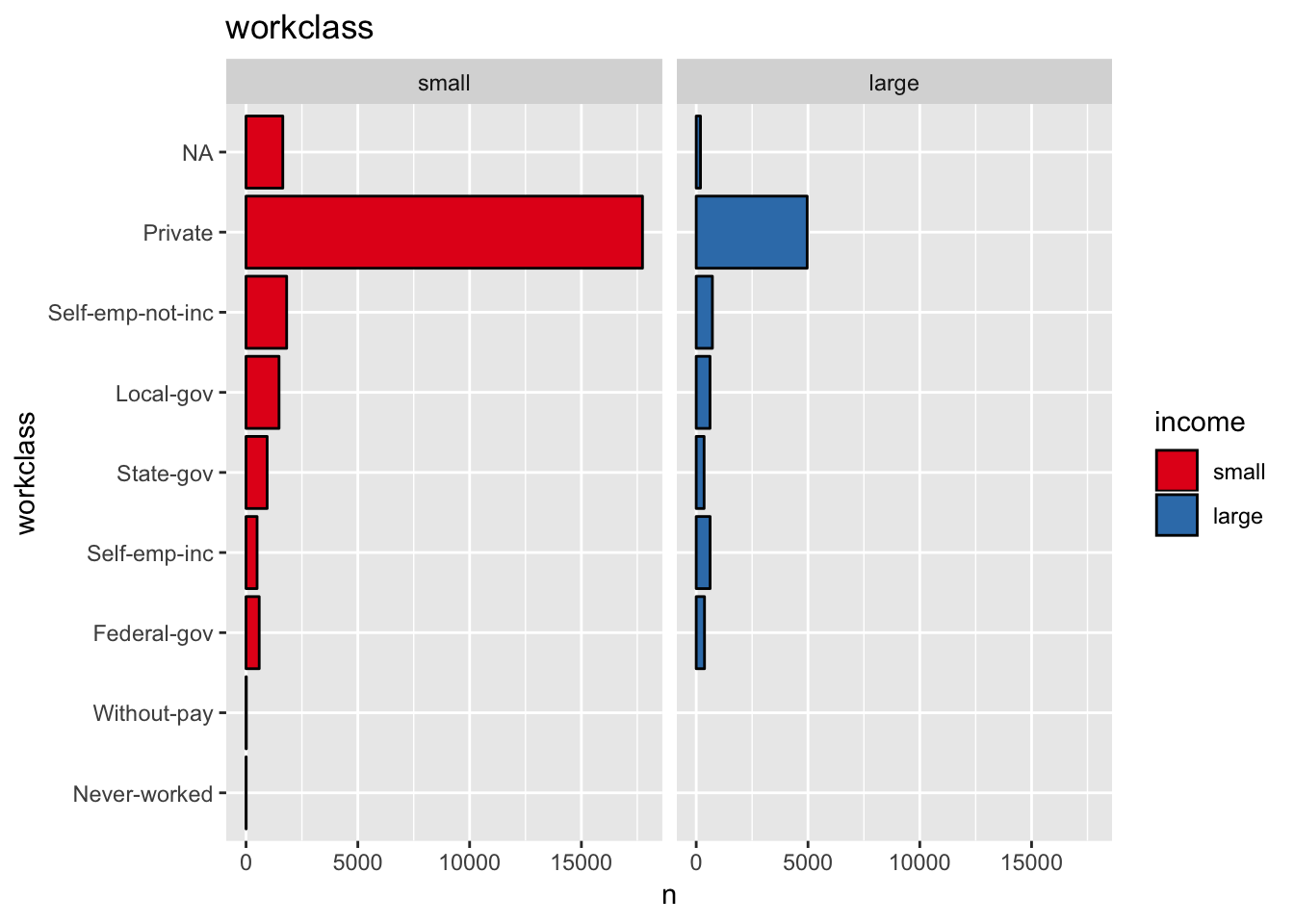

get_stacked_bar_plot <- function(df, var_name, group_var_name, sort_cols = TRUE) {
  
  var_name_sym <- rlang::sym(var_name)
  group_var_name_sym <- rlang::sym(group_var_name)
  
  count_df <- df %>% count(!!var_name_sym, !!group_var_name_sym) 
  
  if (sort_cols) {
    count_df %<>% mutate(!!var_name_sym  := reorder(!!var_name_sym , n))
  }
  
  count_df %>% 
    ggplot(mapping = aes(x = !!var_name_sym, y = n, fill = !!group_var_name_sym)) +
    geom_bar(stat = "identity", color = "black", position = "fill") + 
    coord_flip() +
    labs(title = glue::glue("{var_name} - Share")) +
    scale_fill_brewer(palette = "Set1")
}

get_stacked_bar_plot(df = data_df, var_name = "workclass", group_var_name = "income")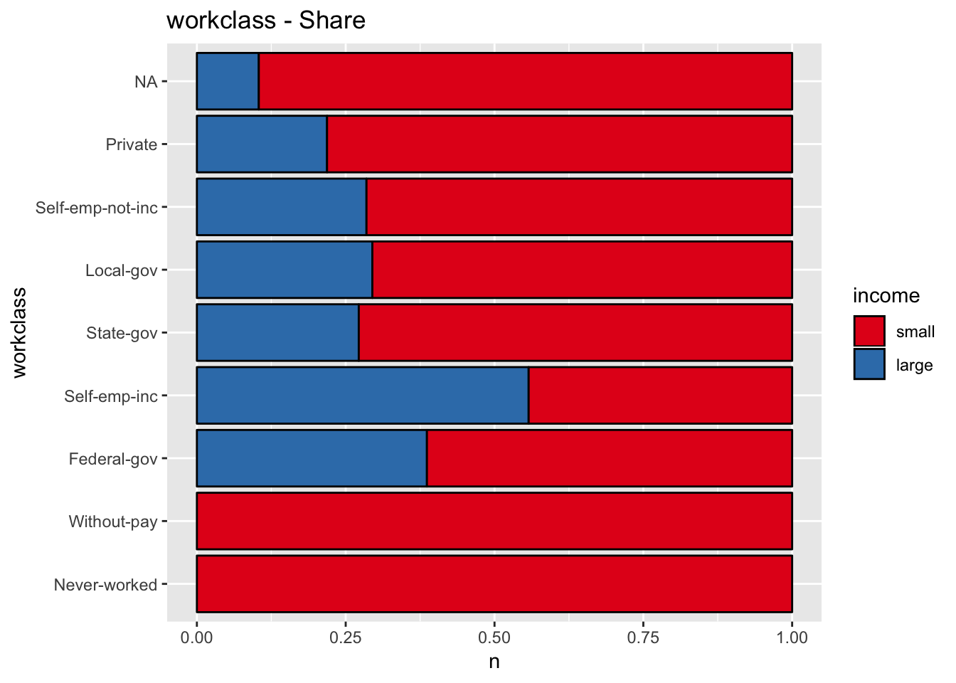

Education

For the education-num plots we keep the ranking on the axis.

get_bar_plot(df = data_df, var_name = "education-num", sort_cols = FALSE)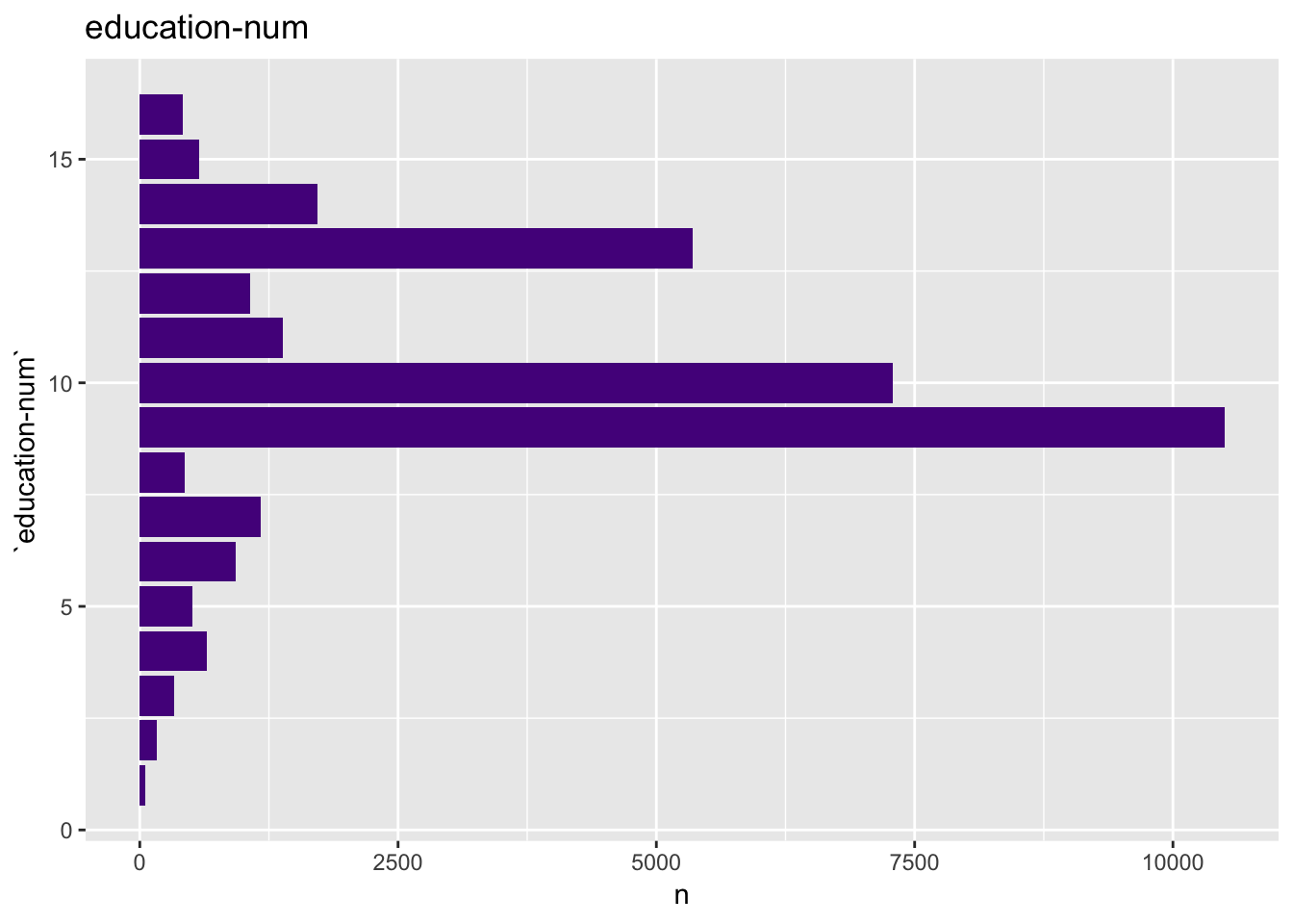

get_split_bar_plot(df = data_df, var_name = "education-num", group_var_name = "income", sort_cols = FALSE)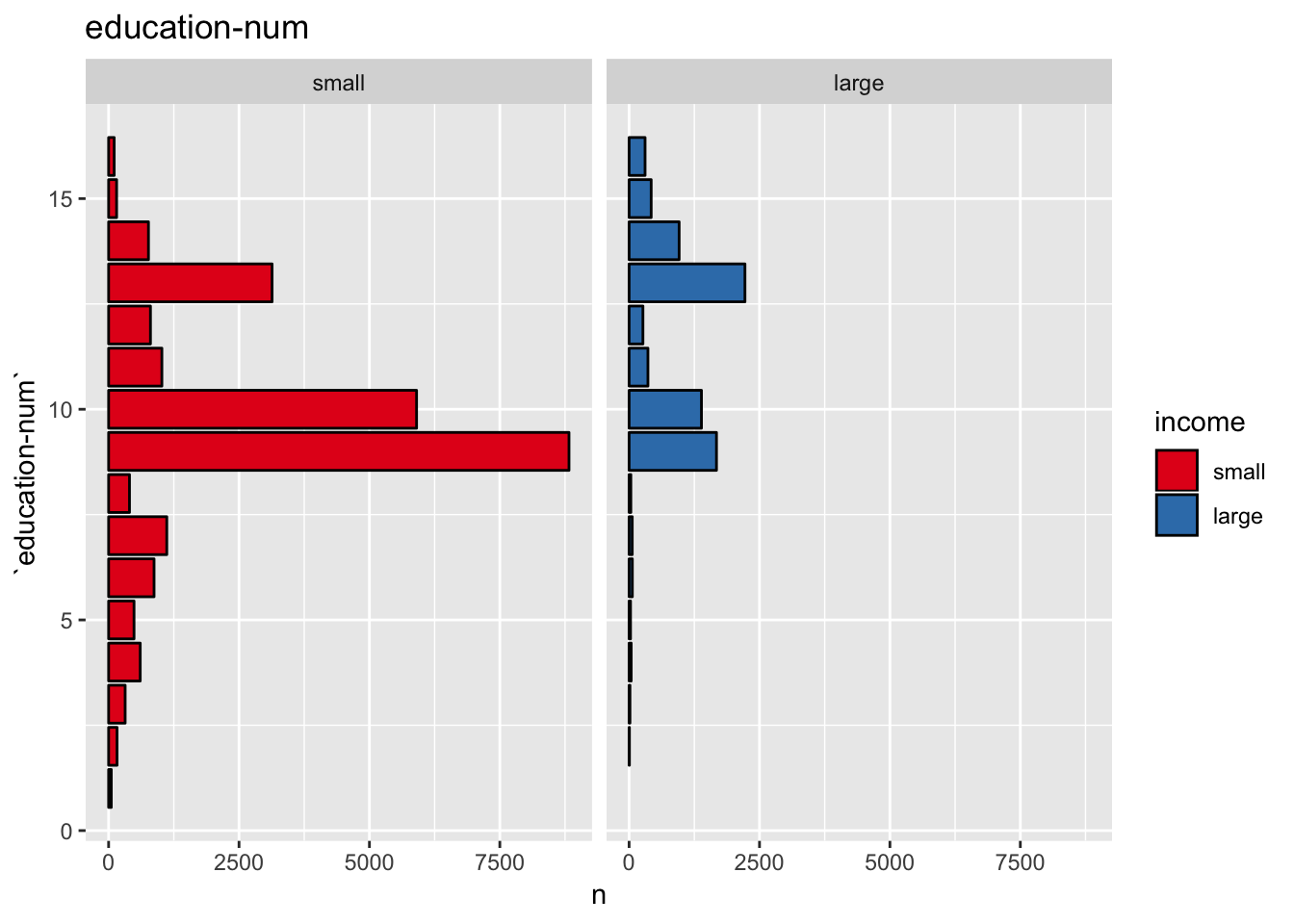

get_stacked_bar_plot(df = data_df, var_name = "education-num", group_var_name = "income", sort_cols = FALSE)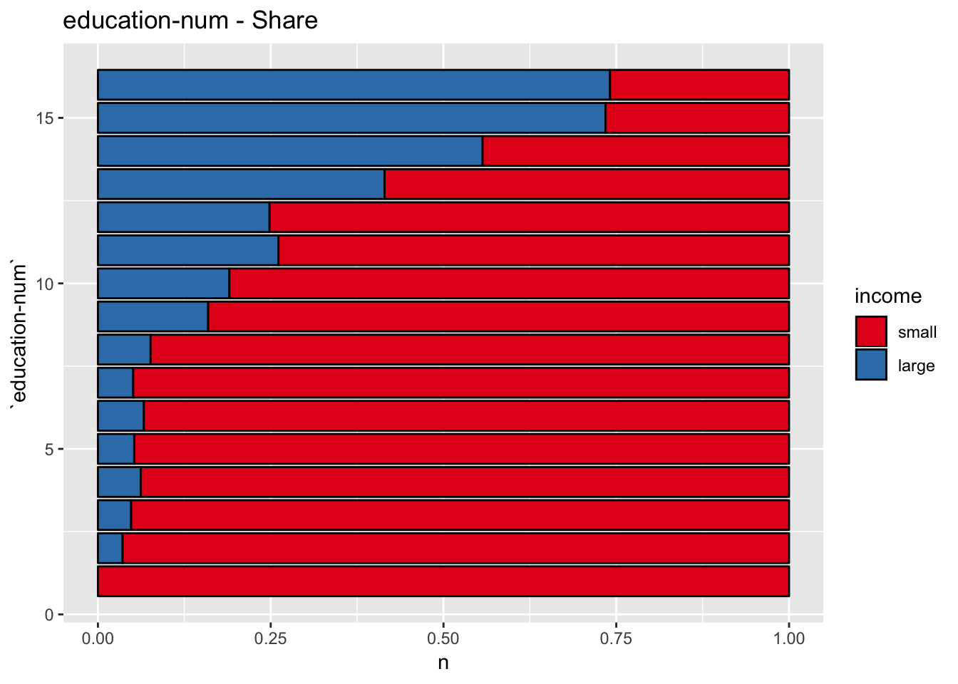

This plot shows that education-num might be a good predictor.

Marital Status

get_bar_plot(df = data_df, var_name = "marital-status")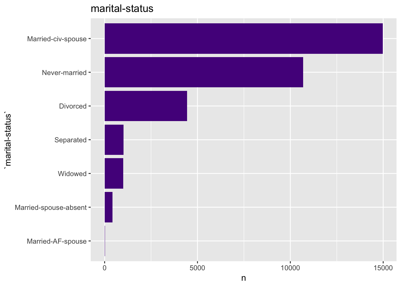

get_split_bar_plot(df = data_df, var_name = "marital-status", group_var_name = "income")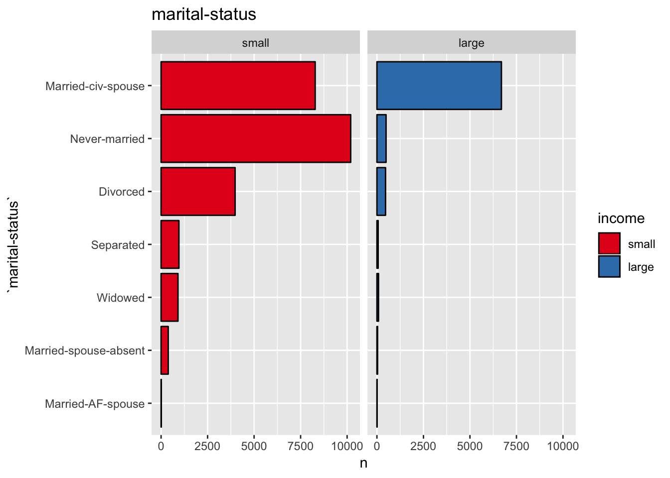

get_stacked_bar_plot(df = data_df, var_name = "marital-status", group_var_name = "income")

Occupation

get_bar_plot(df = data_df, var_name = "occupation")

get_split_bar_plot(df = data_df, var_name = "occupation", group_var_name = "income")

get_stacked_bar_plot(df = data_df, var_name = "occupation", group_var_name = "income")

Relationship

get_bar_plot(df = data_df, var_name = "relationship")

get_split_bar_plot(df = data_df, var_name = "relationship", group_var_name = "income")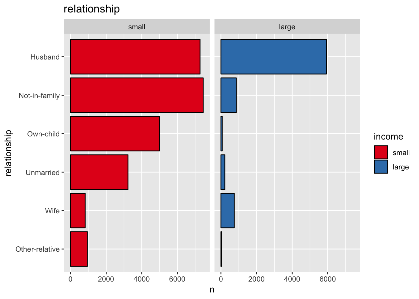

get_stacked_bar_plot(df = data_df, var_name = "relationship", group_var_name = "income")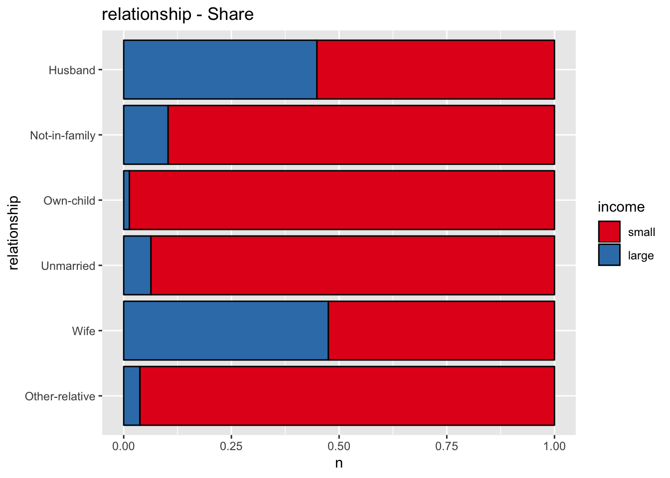

Race

get_bar_plot(df = data_df, var_name = "race")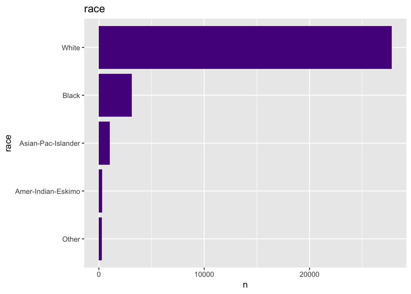

get_split_bar_plot(df = data_df, var_name = "race", group_var_name = "income")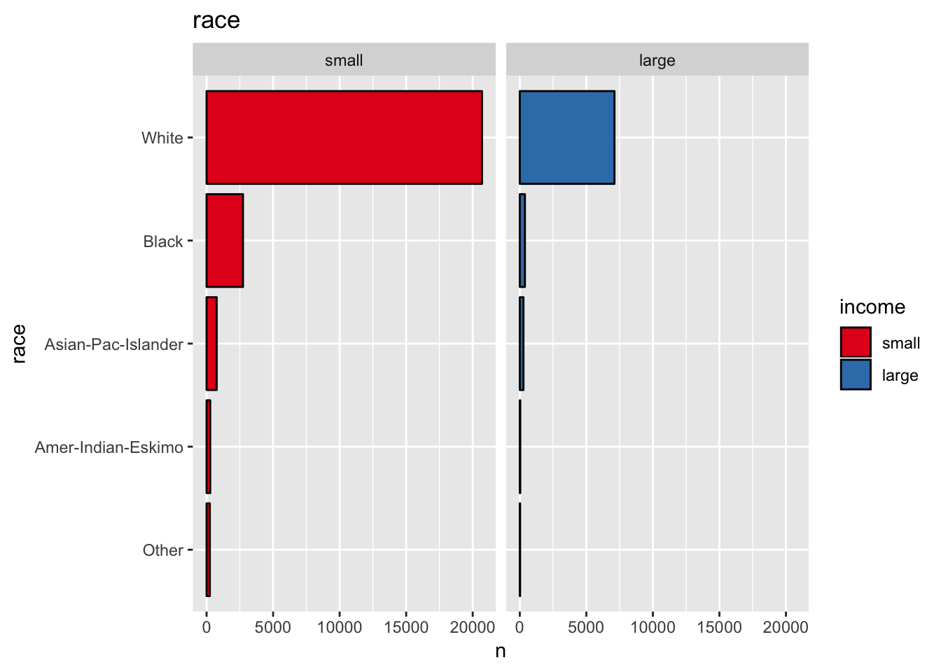

get_stacked_bar_plot(df = data_df, var_name = "race", group_var_name = "income")

get_bar_plot(df = data_df, var_name = "sex")

get_split_bar_plot(df = data_df, var_name = "sex", group_var_name = "income")

get_stacked_bar_plot(df = data_df, var_name = "sex", group_var_name = "income")

The variable sex might also be a good predictor.

Capital Gain

We transform the capital-gain and capital-loss via $x\mapsto \log(x + 1)$ to overcome the skewness of their distribution.

data_df %>% 
  ggplot(mapping = aes(x = log(`capital-gain` + 1), y = ..density.., fill = income)) +
  geom_density(alpha = 0.8) +
  labs(title = "Log Capital Gain") +
  scale_fill_brewer(palette = "Set1")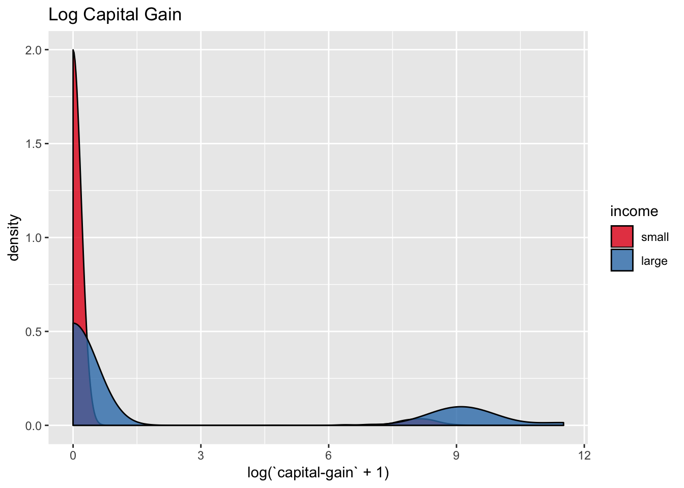

data_df %>% 
  ggplot(mapping = aes(x = log(`capital-gain` + 1), y = age, fill = income)) +
  geom_boxplot() +
  labs(title = "Log Capital Gain") +
  scale_fill_brewer(palette = "Set1")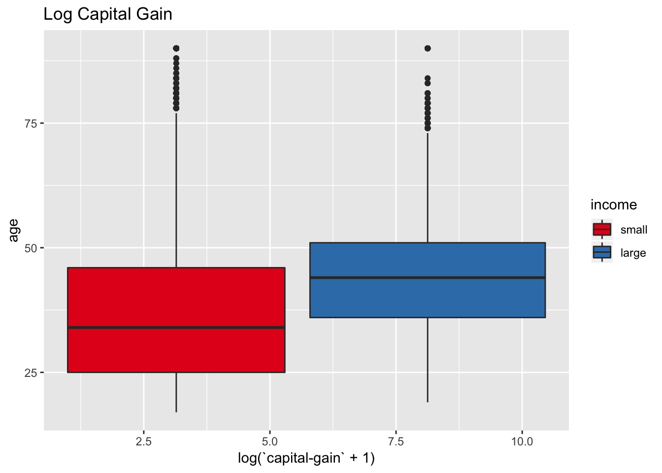

Capital Loss

data_df %>% 
  ggplot(mapping = aes(x = log(`capital-loss` + 1), y = ..density.., fill = income)) +
  geom_density(alpha = 0.8) +
  labs(title = "Capital Loss") +
  scale_fill_brewer(palette = "Set1")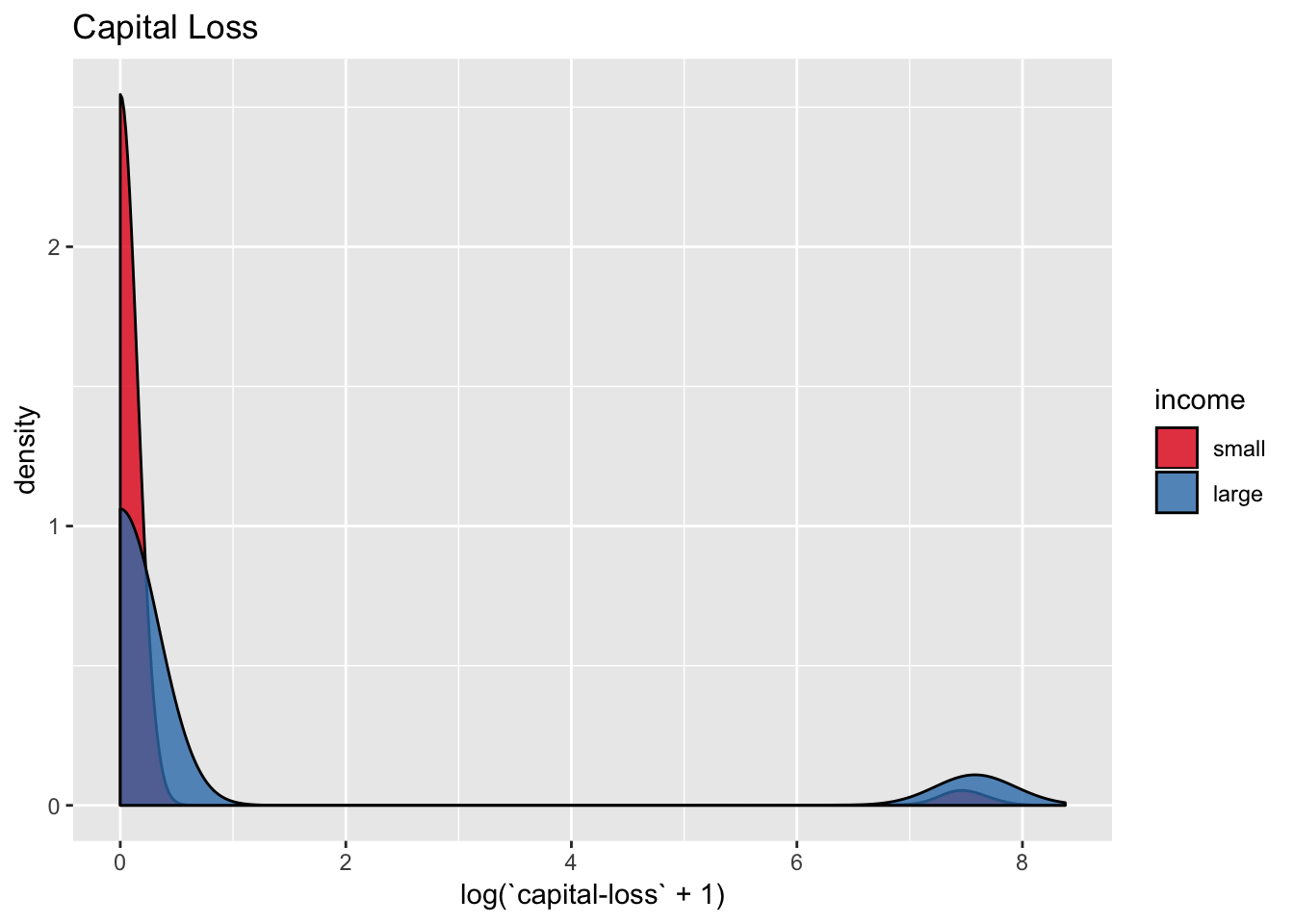

data_df %>% 
  ggplot(mapping = aes(x = log(`capital-loss` + 1), y = age, fill = income)) +
  geom_boxplot() +
  labs(title = "Log Capital Loss") +
  scale_fill_brewer(palette = "Set1")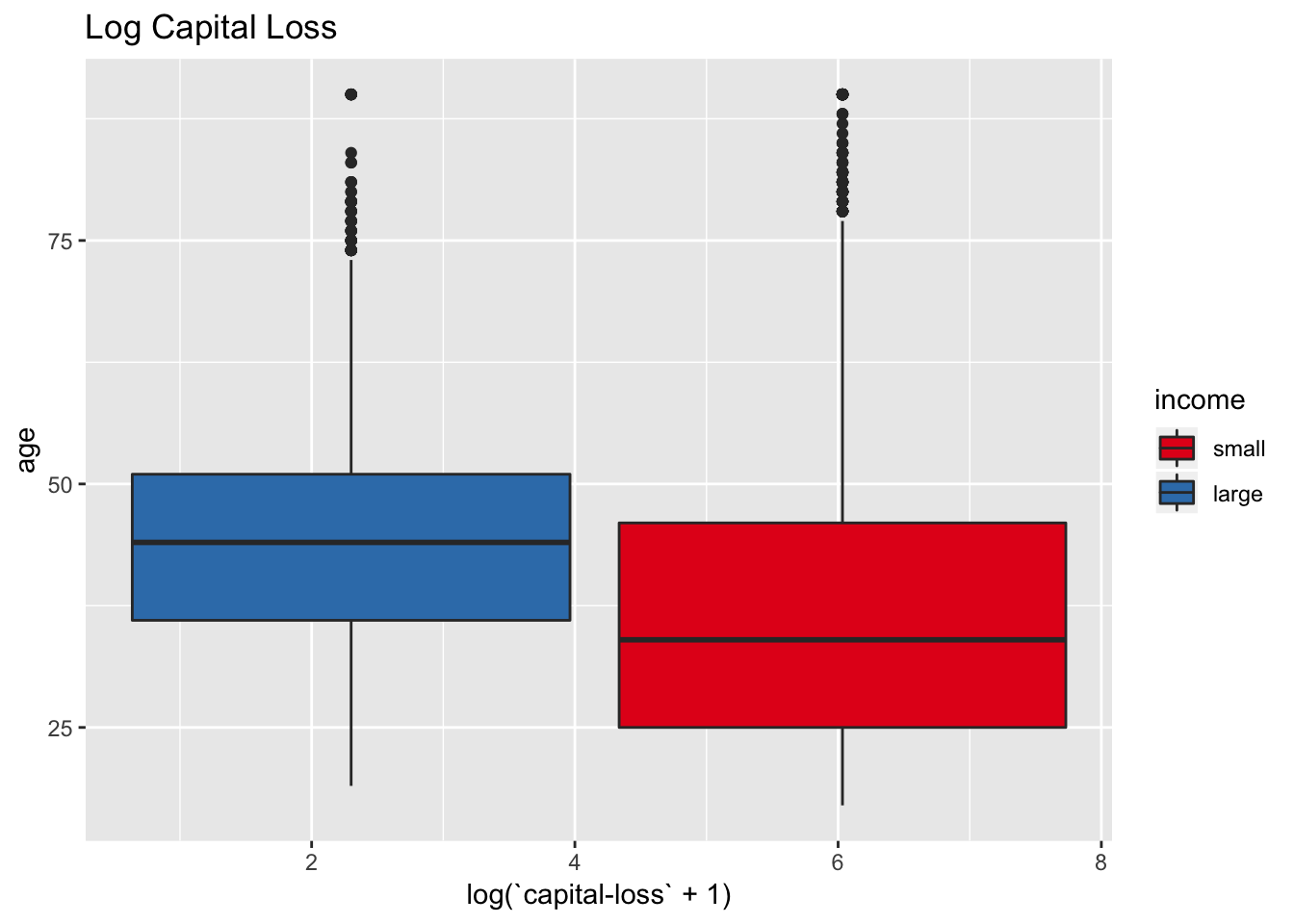

Hours per Week

data_df %>% 
  ggplot(mapping = aes(x = `hours-per-week`, y = ..density.., fill = income)) +
  geom_density(alpha = 0.5) +
  labs(title = "Hours per Week") +
  scale_fill_brewer(palette = "Set1")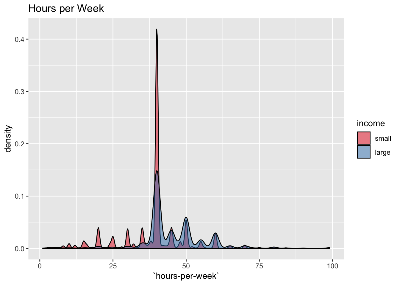

data_df %>% 
  ggplot(mapping = aes(x = `hours-per-week`, y = age, fill = income)) +
  geom_boxplot() +
  labs(title = "Hours per Week") +
  scale_fill_brewer(palette = "Set1")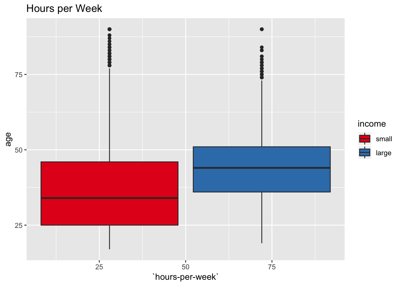

Feature Engineering

We save the transformations into a function (to be applied to new data).

transform_data <- function (df) {
  
  output_df <- df %>% 
    mutate(capital_gain_log = log(`capital-gain` + 1), 
           capital_loss_log = log(`capital-loss` + 1)) %>% 
    select(- `capital-gain`, - `capital-loss`) %>% 
    drop_na()
  
  return(output_df)
}

df <- transform_data(df = data_df)

Next, we format the data so that it is usable for machine learning models.

format_data <- function (df) {
  
  # Define observation matrix and target vector. 
  X <- df %>% select(- income)
  y <- df %>% pull(income) %>% fct_rev()
  
  # Add dummy variables. 
  dummy_obj <- dummyVars("~ .", data = X, sep = "_")
  
  X <- predict(object = dummy_obj, newdata = X) %>% as_tibble()
  
  # Remove predictors with near zero variance. 
  cols_to_rm <- colnames(X)[nearZeroVar(x = X, freqCut = 5000)]
  
  X %<>% select(- cols_to_rm) 
  
  return(list(X = X, y = y))
}

format_data_list <- format_data(df = df)

X <- format_data_list$X
y <- format_data_list$y

# Add function to model list. 
model_list$functions$transform_data <- transform_data
model_list$functions$format_data <- format_data

Data Split

Let us now split the data. We are interested in generating three partitions:

Training Set: Data to fit the model.
Evaluation Set: Data used post-processing techniques.
Test Set: Data used to evaluate model performance.

# Set seed to make results reproducible. 
seed <- 1 
set.seed(seed = seed)
model_list$seed <- seed

split_data <- function (X, y) {
  
  # Split train - other
  split_index_1 <- createDataPartition(y = y, p = 0.7)$Resample1
  
  X_train <- X[split_index_1, ]
  y_train <- y[split_index_1]
  
  X_other <- X[- split_index_1, ]
  y_other <- y[- split_index_1]
  
  split_index_2 <- createDataPartition(y = y_other, p = 1/3)$Resample1
  
  # Split evaluation - test
  X_eval <- X_other[split_index_2, ]
  y_eval <- y_other[split_index_2]
  
  X_test <- X_other[- split_index_2, ]
  y_test <- y_other[- split_index_2]
  
  output_list <- list(
    
    X_train = X_train,
    y_train = y_train, 
    X_eval = X_eval,
    y_eval = y_eval, 
    X_test = X_test,
    y_test = y_test
    
  )
  
  return(output_list)
}

split_data_list <- split_data(X = X, y = y)

X_train <- split_data_list$X_train
y_train <- split_data_list$y_train

X_eval <- split_data_list$X_eval
y_eval <- split_data_list$y_eval

X_test <- split_data_list$X_test
y_test <- split_data_list$y_test

# Add function to model list. 
model_list$functions$split_data <- split_data

Performance Metrics

Before the model fit process, let us briefly recall some common performance metrics for classification problems.

Confision Matrix

C ondition Positive C ondition Negative

Prediction Positive TP FP

Prediction Negative FN TN
- TP = True Positive
- TN = True Negative
- FP = False Positive
- FN = False Negative
- N = TP + TN + FP + FN
Accuracy

C	ondition Positive C	ondition Negative
Prediction Positive	TP	FP
Prediction Negative	FN	TN

\[ \text{acc} = \frac{TP + TN}{N} \]

Kappa

\[ \kappa = \frac{p_o - p_e}{1 - p_e} \] where

$p_e$ = Expected Accuracy (random chance).
$p_o$ = Observed Accuracy.

The kappa metric can be thought as a modification of the accuracy metric based on the class proportions.

Sensitivity (= Recall)

\[ \text{sens} = \frac{TP}{TP + FN} \]

Specitivity

\[ \text{spec} = \frac{TN}{TN + FP} \]

Precision

\[ \text{prec} = \frac{TP}{TP + FP} \]

$F_\beta$

\[ F_\beta = (1 + \beta^2)\frac{\text{prec}\times \text{recall}}{\beta^2\text{prec} + \text{recall}} \]

This metric refers to the area under the curve of the ROC curve, which is created by plotting the true positive rate (= sensitivity) against the false positive rate (1 − specificity) at various propability threshold. The AUC does not depend on the cutoff probability threshold for the predicted classes.

Prediction Models

Next, we are going to train various machine learning models to compare performance and explore some techniques to overcome the class imbalance problem. We will start with very simple models in order to benchmark the performance metrics discussed above.

Trivial Model

Let us consider the model which always predicts income = small.

y_pred_trivial <- map_chr(.x = y_test, .f = ~ "small") %>% 
  as_factor(ordered = TRUE, levels = c("small", "large"))

# Confusion Matrix. 
conf_matrix_trivial <-  confusionMatrix(data = y_pred_trivial, reference =  y_test)
conf_matrix_trivial

## Confusion Matrix and Statistics
## 
##           Reference
## Prediction large small
##      large     0     0
##      small  1530  4613
##                                           
##                Accuracy : 0.7509          
##                  95% CI : (0.7399, 0.7617)
##     No Information Rate : 0.7509          
##     P-Value [Acc > NIR] : 0.5069          
##                                           
##                   Kappa : 0               
##                                           
##  Mcnemar's Test P-Value : <2e-16          
##                                           
##             Sensitivity : 0.0000          
##             Specificity : 1.0000          
##          Pos Pred Value :    NaN          
##          Neg Pred Value : 0.7509          
##              Prevalence : 0.2491          
##          Detection Rate : 0.0000          
##    Detection Prevalence : 0.0000          
##       Balanced Accuracy : 0.5000          
##                                           
##        'Positive' Class : large           
##

Note that the accuracy is 0.75. Nevertheless, both kappa and the senitivity metrics vanish. Let us see the ROC curve:

roc_curve_trivial <- roc(response = y_test, predictor = rep(0, length(y_pred_trivial)))

auc_trivial <- roc_curve_trivial %>% 
  auc() %>% 
  round(digits = 3)

plot(roc_curve_trivial)
title(main = str_c("Trivial Model - ROC AUC (Test Set) = ", auc_trivial), line = 2.5)

Random Model

Next, Let us now generate random predictions based on the proportion of the target variable.

prop <- sum(y_train == "large") / length(y_train)

y_pred_random_num <- rbernoulli(n = length(y_test), p = prop) %>% as.numeric()

y_pred_random <- y_pred_random_num %>% 
  map_chr(.f = ~ ifelse(test = (.x == 0), yes = "small", no = "large")) %>% 
  as_factor(ordered = TRUE, levels = c("small", "large"))

# Confusion Matrix. 
conf_matrix_random <-  confusionMatrix(data = y_pred_random, reference =  y_test)
conf_matrix_random

## Confusion Matrix and Statistics
## 
##           Reference
## Prediction large small
##      large   376  1140
##      small  1154  3473
##                                           
##                Accuracy : 0.6266          
##                  95% CI : (0.6143, 0.6387)
##     No Information Rate : 0.7509          
##     P-Value [Acc > NIR] : 1.0000          
##                                           
##                   Kappa : -0.0014         
##                                           
##  Mcnemar's Test P-Value : 0.7861          
##                                           
##             Sensitivity : 0.24575         
##             Specificity : 0.75287         
##          Pos Pred Value : 0.24802         
##          Neg Pred Value : 0.75059         
##              Prevalence : 0.24906         
##          Detection Rate : 0.06121         
##    Detection Prevalence : 0.24678         
##       Balanced Accuracy : 0.49931         
##                                           
##        'Positive' Class : large           
##

Note that the accuracy in this case is 0.63 (still above 0.5). Also, we see how this random model has a non-vanishing sensitivity. Moreover, note that the sentitivity and specificity concide (approximately) with the parameter prop and 1 - prop respectively.

roc_curve_random <- roc(response = y_test, predictor = y_pred_random_num)

auc_random <- roc_curve_random %>% 
  auc() %>% 
  round(digits = 3)

plot(roc_curve_random)
title(main = str_c("Random Model - ROC AUC (Train) = ", auc_random), line = 2.5)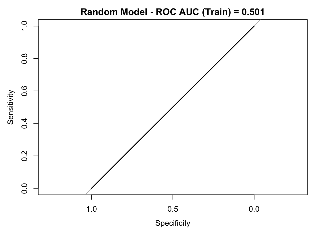

Set Sampling Method

Now we want to train models with non-trivial prediction power. In order to avoid overfitting, we are going to define a cross-validation schema.

# We use the same wrapper functions for the summara functions as Section 16.9 (Computing)

 five_stats <- function (...) {
  
  c(twoClassSummary(...), defaultSummary(...))
  
}

four_stats <- function (data, lev = levels(data$obs), model = NULL) {
  
  acc_kapp <- postResample(pred = data[, "pred"], obs = data[, "obs"])
  
  out <- c(
    acc_kapp, 
    sensitivity(pred = data[, "pred"], obs = data[, "obs"], reference = lev[1]), 
    specificity(pred = data[, "pred"], obs = data[, "obs"], reference = lev[2])
  )
  
  names(out)[3:4] <- c("Sens", "Spec")
  
  return(out)
}

# Define cross validation.
cv_num <- 7

train_control <- trainControl(method = "cv",
                              number = cv_num,
                              classProbs = TRUE, 
                              summaryFunction = five_stats,
                              allowParallel = TRUE, 
                              verboseIter = FALSE)

# Change summaryFunction and set classProbs = False. 
train_control_no_prob <- train_control
train_control_no_prob$summaryFunction <- four_stats
train_control_no_prob$classProbs <- FALSE

PLS + Logistic Regression

The first model we are going to train is a logistic regression. As we might have multicollinearity, we run partial least squares to reduce the dimension of the predictor space (we also scale and center). The number of components to select is an hyperparameter which we tune via cross-validation. Let us select Accuracy as the metric to evaluate model performance.

# Parallel Computation.
cl <- makePSOCKcluster(detectCores())
registerDoParallel(cl)

# Train model.
pls_model_1 <- train(x = X_train,
                     y = y_train,
                     method = "pls",
                     family = binomial(link = "logit"), 
                     tuneLength = 10,
                     preProcess = c("scale", "center"), 
                     trControl = train_control,
                     metric = "Accuracy")

stopCluster(cl)

model_list$models <- list(pls_model_1 = pls_model_1)
pls_model_1

## Partial Least Squares 
## 
## 21503 samples
##    46 predictor
##     2 classes: 'large', 'small' 
## 
## Pre-processing: scaled (46), centered (46) 
## Resampling: Cross-Validated (7 fold) 
## Summary of sample sizes: 18432, 18431, 18431, 18431, 18431, 18431, ... 
## Resampling results across tuning parameters:
## 
##   ncomp  ROC        Sens       Spec       Accuracy   Kappa    
##    1     0.8715987  0.5107376  0.9254398  0.8221649  0.4783562
##    2     0.8916595  0.5563025  0.9318183  0.8383022  0.5302204
##    3     0.8917140  0.5587302  0.9311372  0.8383951  0.5312680
##    4     0.8921241  0.5507003  0.9337382  0.8383488  0.5283604
##    5     0.8921858  0.5493931  0.9343574  0.8384883  0.5282131
##    6     0.8923291  0.5495798  0.9341717  0.8383953  0.5280845
##    7     0.8923789  0.5495798  0.9342955  0.8384883  0.5282878
##    8     0.8923168  0.5499533  0.9341098  0.8384418  0.5283179
##    9     0.8923396  0.5495798  0.9341717  0.8383953  0.5280920
##   10     0.8922221  0.5497666  0.9343575  0.8385813  0.5285589
## 
## Accuracy was used to select the optimal model using the largest value.
## The final value used for the model was ncomp = 10.

Let us plot the cross-valitation results:

plot(pls_model_1)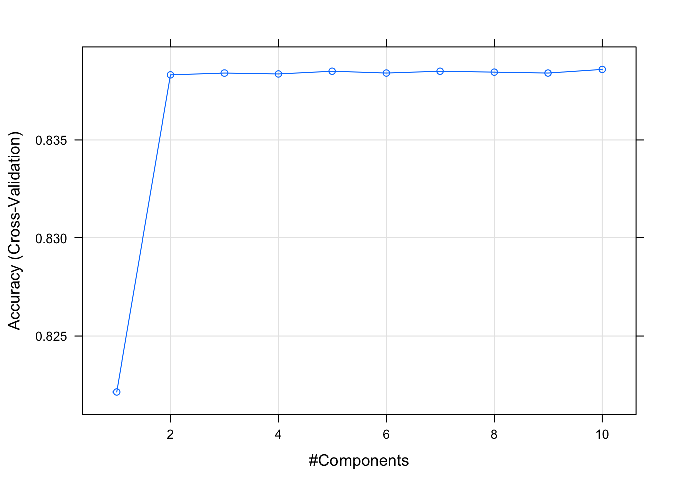

# Number of components. 
pls_model_1$finalModel$ncomp

## [1] 10

Let us generate predictions on the test set.

get_pred_df <- function(model_obj, X_test, y_test, threshold = 0.5) {
  
  y_pred_num <- predict(object = model_obj, newdata = X_test, type = "prob") %>% pull(large)
  
  y_pred <- y_pred_num %>% 
    map_chr(.f = ~ ifelse(test = .x > threshold, yes = "large", no = "small")) %>% 
    as_factor()

  pred_df <- tibble(
    y_test = y_test,  
    y_test_num = map_dbl(.x = y_test, 
                         .f =  ~ ifelse(test = (.x == "small"), yes = 0, no = 1)), 
    y_pred = y_pred, 
    y_pred_num
  )
  
  return(pred_df)
}

pred_df <- get_pred_df(model_obj = pls_model_1, X_test = X_test, y_test = y_test)
# Confusion Matrix. 
conf_matrix_test <- confusionMatrix(data = pred_df$y_pred, reference =  y_test)
conf_matrix_test

## Confusion Matrix and Statistics
## 
##           Reference
## Prediction large small
##      large   844   312
##      small   686  4301
##                                           
##                Accuracy : 0.8375          
##                  95% CI : (0.8281, 0.8467)
##     No Information Rate : 0.7509          
##     P-Value [Acc > NIR] : < 2.2e-16       
##                                           
##                   Kappa : 0.5271          
##                                           
##  Mcnemar's Test P-Value : < 2.2e-16       
##                                           
##             Sensitivity : 0.5516          
##             Specificity : 0.9324          
##          Pos Pred Value : 0.7301          
##          Neg Pred Value : 0.8624          
##              Prevalence : 0.2491          
##          Detection Rate : 0.1374          
##    Detection Prevalence : 0.1882          
##       Balanced Accuracy : 0.7420          
##                                           
##        'Positive' Class : large           
##

Note that the sensitivity is around 0.56. This shows that this model does is very conservative when trying to predict a large label. Let us see this through the predicted distributions.

pred_df %>% 
  ggplot(mapping = aes(x = y_test, y = y_pred_num, fill = y_test)) +
  geom_boxplot() + 
  geom_abline(slope = 0, 
              intercept = 0.5, 
              alpha = 0.8, 
              linetype = 2, 
              color = "purple4") +
  scale_fill_brewer(palette = "Set1", direction = -1) +
  labs(title = "Preditcted Distributions - PLS Model 1 (Max Accuracy)", 
       subtitle = "Prediction Cut = 0.5", 
       x = "test label", 
       y = "predicted probability") +
  scale_x_discrete(limits = rev(levels(y_test)))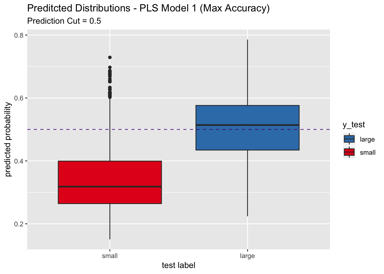

roc_curve_test <- roc(response = y_test, 
                      pred_df$y_pred_num, 
                      levels = c("small", "large"))

auc_pls <- roc_curve_test %>% 
  auc() %>% 
  round(digits = 3)

plot(roc_curve_test)
title(main = str_c("PLS Model 1 - ROC AUC (Test) = ", auc_pls), line = 2.5)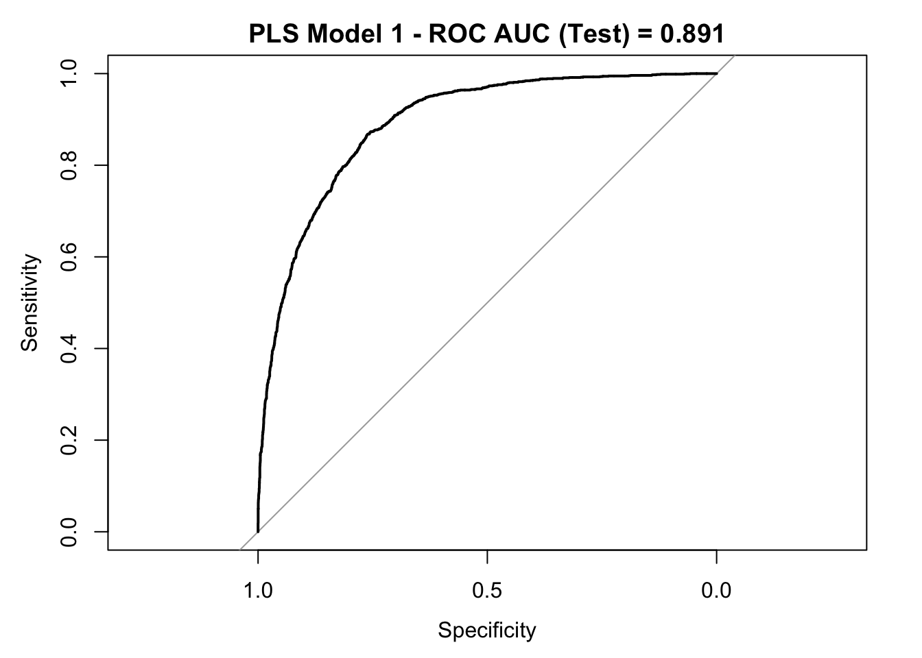

Generalized Boosted Regression Model (GBM)

Now we consider a boosted tree model (stochastic gradient boosting), see gbm. There are some hyperparameters to tune:

n.trees
interaction.depth
shrinkage (kept constant)
n.minobsinnode(kept constant)

# Parallel Computation.
cl <- makePSOCKcluster(detectCores())
registerDoParallel(cl)

# Train model.
gbm_model_1 <- train(x = X_train,
                     y = y_train,
                     method = "gbm",
                     tuneLength = 7,
                     trControl = train_control,
                     metric = "Accuracy", 
                     verbose = FALSE)

stopCluster(cl)

model_list$models$gbm_model_1 <- gbm_model_1
gbm_model_1

## Stochastic Gradient Boosting 
## 
## 21503 samples
##    46 predictor
##     2 classes: 'large', 'small' 
## 
## No pre-processing
## Resampling: Cross-Validated (7 fold) 
## Summary of sample sizes: 18431, 18431, 18432, 18431, 18431, 18431, ... 
## Resampling results across tuning parameters:
## 
##   interaction.depth  n.trees  ROC        Sens       Spec       Accuracy 
##   1                   50      0.8928287  0.4623716  0.9651344  0.8399291
##   1                  100      0.9020806  0.5262372  0.9559694  0.8489510
##   1                  150      0.9058479  0.5437908  0.9516343  0.8500670
##   1                  200      0.9085090  0.5579832  0.9498385  0.8522528
##   1                  250      0.9103367  0.5706816  0.9474852  0.8536479
##   1                  300      0.9114115  0.5788982  0.9458133  0.8544385
##   1                  350      0.9123269  0.5887955  0.9438317  0.8554152
##   2                   50      0.9023472  0.5348273  0.9541737  0.8497417
##   2                  100      0.9092874  0.5643324  0.9500244  0.8539735
##   2                  150      0.9132127  0.5845005  0.9463707  0.8562523
##   2                  200      0.9153963  0.5992530  0.9427170  0.8571823
##   2                  250      0.9170762  0.6078431  0.9416641  0.8585309
##   2                  300      0.9180450  0.6134454  0.9407353  0.8592285
##   2                  350      0.9189936  0.6203548  0.9406734  0.8609027
##   3                   50      0.9065395  0.5462185  0.9528110  0.8515552
##   3                  100      0.9140924  0.5867414  0.9457514  0.8563453
##   3                  150      0.9174196  0.6070962  0.9427789  0.8591821
##   3                  200      0.9190822  0.6181139  0.9411068  0.8606702
##   3                  250      0.9202552  0.6242764  0.9393109  0.8608561
##   3                  300      0.9209524  0.6276377  0.9388776  0.8613678
##   3                  350      0.9216507  0.6332400  0.9383822  0.8623909
##   4                   50      0.9099694  0.5665733  0.9502721  0.8547175
##   4                  100      0.9168304  0.6035481  0.9437079  0.8589961
##   4                  150      0.9195390  0.6220355  0.9416024  0.8620189
##   4                  200      0.9209090  0.6304388  0.9398684  0.8628094
##   4                  250      0.9219047  0.6362278  0.9393112  0.8638326
##   4                  300      0.9223488  0.6405229  0.9385680  0.8643442
##   4                  350      0.9229375  0.6455649  0.9393731  0.8662044
##   5                   50      0.9122942  0.5725490  0.9481046  0.8545781
##   5                  100      0.9186557  0.6149393  0.9426552  0.8610422
##   5                  150      0.9209015  0.6287582  0.9405496  0.8629024
##   5                  200      0.9220614  0.6377218  0.9393731  0.8642511
##   5                  250      0.9224993  0.6464986  0.9401164  0.8669951
##   5                  300      0.9226629  0.6463119  0.9394972  0.8664835
##   5                  350      0.9228012  0.6485528  0.9388779  0.8665766
##   6                   50      0.9138177  0.5886088  0.9466185  0.8574614
##   6                  100      0.9194991  0.6227824  0.9404258  0.8613213
##   6                  150      0.9214319  0.6367880  0.9394350  0.8640651
##   6                  200      0.9228085  0.6451914  0.9386920  0.8655999
##   6                  250      0.9228065  0.6479925  0.9381346  0.8658789
##   6                  300      0.9229573  0.6491130  0.9368959  0.8652279
##   6                  350      0.9231076  0.6524743  0.9367103  0.8659255
##   7                   50      0.9151054  0.5979458  0.9447607  0.8583915
##   7                  100      0.9210021  0.6315593  0.9399303  0.8631349
##   7                  150      0.9227249  0.6399627  0.9381966  0.8639257
##   7                  200      0.9230369  0.6461251  0.9384442  0.8656464
##   7                  250      0.9233549  0.6504202  0.9367102  0.8654138
##   7                  300      0.9232540  0.6515406  0.9357814  0.8649954
##   7                  350      0.9229876  0.6535948  0.9342952  0.8643909
##   Kappa    
##   0.4995521
##   0.5441721
##   0.5527143
##   0.5624267
##   0.5696923
##   0.5740783
##   0.5793498
##   0.5489243
##   0.5684390
##   0.5800005
##   0.5865894
##   0.5922634
##   0.5954897
##   0.6013071
##   0.5569838
##   0.5808921
##   0.5934703
##   0.6001158
##   0.6023542
##   0.6044653
##   0.6083782
##   0.5708563
##   0.5920418
##   0.6043377
##   0.6085388
##   0.6124479
##   0.6148621
##   0.6204834
##   0.5724564
##   0.6000462
##   0.6083179
##   0.6138885
##   0.6225199
##   0.6212895
##   0.6221080
##   0.5840397
##   0.6029512
##   0.6131621
##   0.6190100
##   0.6203975
##   0.6192112
##   0.6216878
##   0.5889798
##   0.6096210
##   0.6137509
##   0.6193474
##   0.6199663
##   0.6193113
##   0.6184656
## 
## Tuning parameter 'shrinkage' was held constant at a value of 0.1
## 
## Tuning parameter 'n.minobsinnode' was held constant at a value of 10
## Accuracy was used to select the optimal model using the largest value.
## The final values used for the model were n.trees = 250,
##  interaction.depth = 5, shrinkage = 0.1 and n.minobsinnode = 10.

Let us generate predictions on the test set.

pred_df <- get_pred_df(model_obj = gbm_model_1, X_test = X_test, y_test = y_test)
# Confusion Matrix. 
conf_matrix_test <- confusionMatrix(data = pred_df$y_pred, reference =  y_test)
conf_matrix_test

## Confusion Matrix and Statistics
## 
##           Reference
## Prediction large small
##      large  1002   279
##      small   528  4334
##                                          
##                Accuracy : 0.8686         
##                  95% CI : (0.8599, 0.877)
##     No Information Rate : 0.7509         
##     P-Value [Acc > NIR] : < 2.2e-16      
##                                          
##                   Kappa : 0.6286         
##                                          
##  Mcnemar's Test P-Value : < 2.2e-16      
##                                          
##             Sensitivity : 0.6549         
##             Specificity : 0.9395         
##          Pos Pred Value : 0.7822         
##          Neg Pred Value : 0.8914         
##              Prevalence : 0.2491         
##          Detection Rate : 0.1631         
##    Detection Prevalence : 0.2085         
##       Balanced Accuracy : 0.7972         
##                                          
##        'Positive' Class : large          
##

The accuracy, the sesitivity and specificity are higher that the pls model above. Let us see the predicted distribution on the test set.

pred_df %>% 
  ggplot(mapping = aes(x = y_test, y = y_pred_num, fill = y_test)) +
  geom_boxplot() + 
  geom_abline(slope = 0, 
              intercept = 0.5, 
              alpha = 0.8, 
              linetype = 2, 
              color = "purple4", show.legend = TRUE) +
  scale_fill_brewer(palette = "Set1", direction = -1) +
  labs(title = "Preditcted Distributions - GBM Model 1 (Max Accuracy)", 
       subtitle = "Prediction Cut = 0.5", 
       x = "test label", 
       y = "predicted probability") +
  scale_x_discrete(limits = rev(levels(y_test)))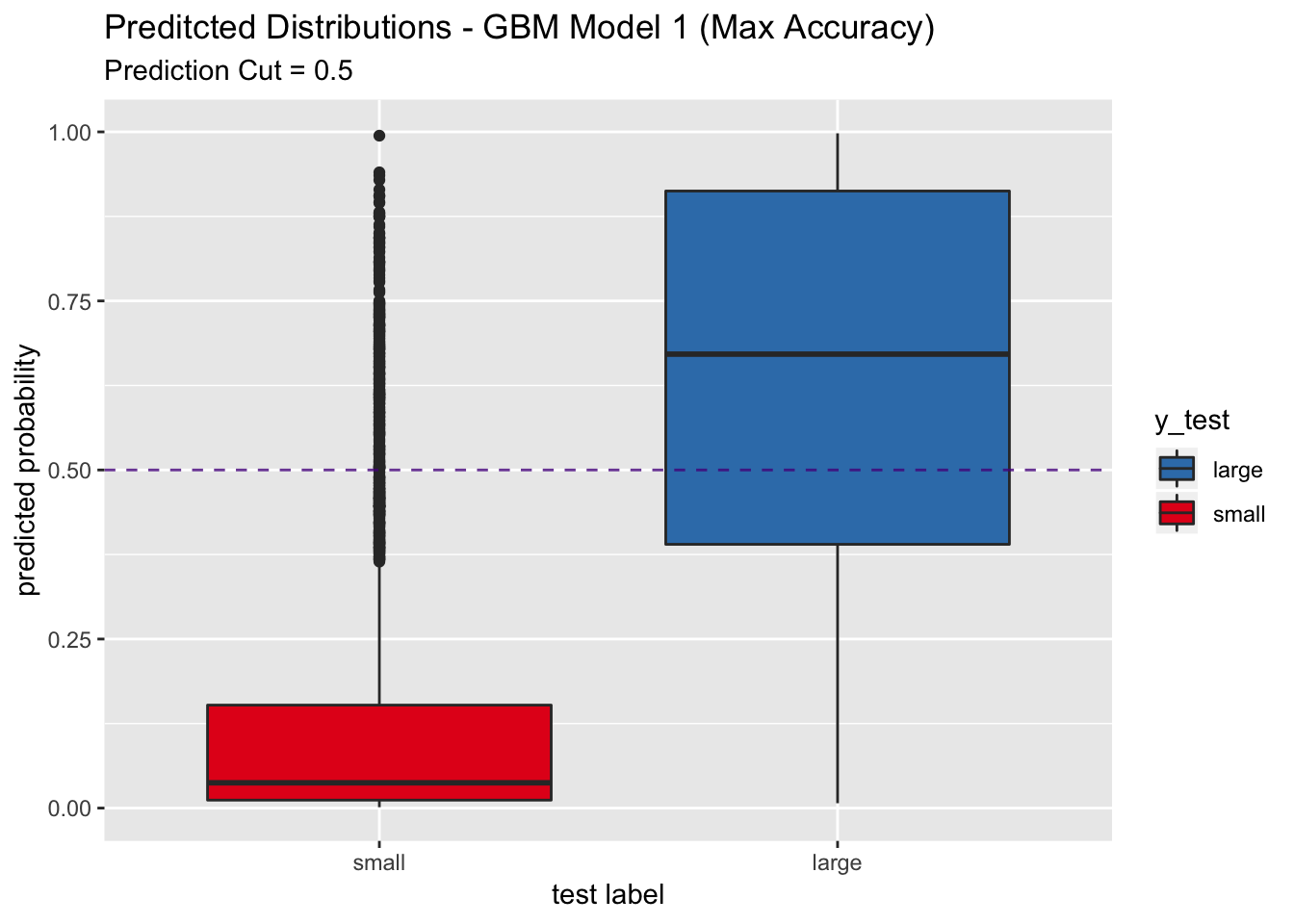

roc_curve_test <- roc(response = y_test, 
                      pred_df$y_pred_num, 
                      levels = c("small", "large"))

auc_gbm <- roc_curve_test %>% 
  auc() %>% 
  round(digits = 3)

plot(roc_curve_test)
title(main = str_c("GBM Model 1 - ROC AUC (Test) = ", auc_gbm), line = 2.5)

Let us compute the variable importance ranking for this model.

gbm_model_1$finalModel %>% 
  varImp() %>% 
  rownames_to_column(var = "Variable") %>% 
  mutate(Overall = Overall / sum(Overall)) %>% 
  mutate(Variable = reorder(Variable, Overall)) %>% 
  arrange(- Overall) %>% 
  head(15) %>% 
  ggplot(mapping = aes(x = Variable, y = Overall)) +
  geom_bar(stat = "identity", fill = "dark green") + 
  ggtitle(label = 'GBM Model 1 -Variable Importance - Top 15') +
  coord_flip()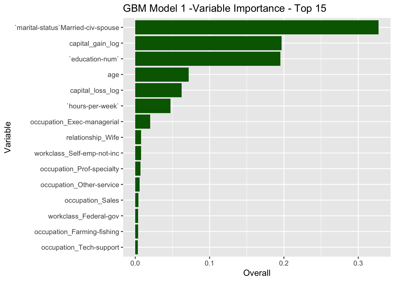

Overall, we see that the gbm model has better metrics than the pls model.

Remedies for Class Imbalance

“The simplest approach to counteracting the negative effects of class imbalance is to tune the model to maximize the accuracy of the minority class” Applied Predictive Modeling, Section 16.3. To do this we set metric = “Sens” in the tain function.

Model Fit - Maximize Sensitivity

PLS Model

# Parallel Computation.
cl <- makePSOCKcluster(detectCores())
registerDoParallel(cl)

# Train model.
pls_model_2 <- train(x = X_train,
                     y = y_train,
                     method = "pls",
                     family = binomial(link = "logit"), 
                     tuneLength = 10,
                     preProcess = c("scale", "center"), 
                     trControl = train_control,
                     metric = "Sens", 
                     verbose = FALSE)

stopCluster(cl)

model_list$models$pls_model_2 = pls_model_2
pls_model_2

## Partial Least Squares 
## 
## 21503 samples
##    46 predictor
##     2 classes: 'large', 'small' 
## 
## Pre-processing: scaled (46), centered (46) 
## Resampling: Cross-Validated (7 fold) 
## Summary of sample sizes: 18431, 18431, 18431, 18431, 18431, 18431, ... 
## Resampling results across tuning parameters:
## 
##   ncomp  ROC        Sens       Spec       Accuracy   Kappa    
##    1     0.8717359  0.5126050  0.9251297  0.8223970  0.4796289
##    2     0.8916039  0.5563025  0.9315703  0.8381157  0.5298420
##    3     0.8915513  0.5589169  0.9310749  0.8383947  0.5313856
##    4     0.8918662  0.5490196  0.9333661  0.8376506  0.5263448
##    5     0.8919885  0.5486461  0.9334900  0.8376506  0.5262041
##    6     0.8921355  0.5484594  0.9336758  0.8377436  0.5263377
##    7     0.8921707  0.5486461  0.9335519  0.8376971  0.5262966
##    8     0.8921095  0.5486461  0.9335519  0.8376971  0.5263026
##    9     0.8921261  0.5477124  0.9339234  0.8377436  0.5260668
##   10     0.8920127  0.5484594  0.9338615  0.8378831  0.5266422
## 
## Sens was used to select the optimal model using the largest value.
## The final value used for the model was ncomp = 3.

Let us see the performance metrics on the test set.

pred_df <- get_pred_df(model_obj = pls_model_2, X_test = X_test, y_test = y_test)
# Confusion Matrix. 
conf_matrix_test <- confusionMatrix(data = pred_df$y_pred, reference =  y_test)
conf_matrix_test

## Confusion Matrix and Statistics
## 
##           Reference
## Prediction large small
##      large   859   313
##      small   671  4300
##                                           
##                Accuracy : 0.8398          
##                  95% CI : (0.8304, 0.8489)
##     No Information Rate : 0.7509          
##     P-Value [Acc > NIR] : < 2.2e-16       
##                                           
##                   Kappa : 0.5355          
##                                           
##  Mcnemar's Test P-Value : < 2.2e-16       
##                                           
##             Sensitivity : 0.5614          
##             Specificity : 0.9321          
##          Pos Pred Value : 0.7329          
##          Neg Pred Value : 0.8650          
##              Prevalence : 0.2491          
##          Detection Rate : 0.1398          
##    Detection Prevalence : 0.1908          
##       Balanced Accuracy : 0.7468          
##                                           
##        'Positive' Class : large           
##

We do not see a significant increase in sensitivity.

Let us plot the predicted probability distributions on the test set.

pred_df %>% 
  ggplot(mapping = aes(x = y_test, y = y_pred_num, fill = y_test)) +
  geom_boxplot() + 
  geom_abline(slope = 0, 
              intercept = 0.5, 
              alpha = 0.8, 
              linetype = 2, 
              color = "purple4", show.legend = TRUE) +
  scale_fill_brewer(palette = "Set1", direction = -1) +
  labs(title = "Preditcted Distributions - PLS Model 2 (Max Sens)", 
       subtitle = "Prediction Cut = 0.5", 
       x = "test label", 
       y = "predicted probability") +
  scale_x_discrete(limits = rev(levels(y_test)))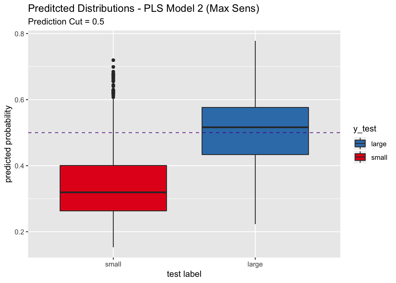

GBM Model

We proceed in a similar way for the gbm model.

# Parallel Computation.
cl <- makePSOCKcluster(detectCores())
registerDoParallel(cl)

# Train model.
gbm_model_2 <- train(x = X_train,
                     y = y_train,
                     method = "gbm",
                     tuneLength = 7,
                     trControl = train_control,
                     metric = "Sens", 
                     verbose = FALSE)

stopCluster(cl)

model_list$models$gbm_model_2 <- gbm_model_2

Let us see the sensitivity as a function of the n.trees and interaction.depth.

gbm_model_2$results %>% 
  ggplot(mapping = aes(x = n.trees, y = Sens, color  = interaction.depth)) +
  geom_point() +
  labs(title = "Model Sensitivity")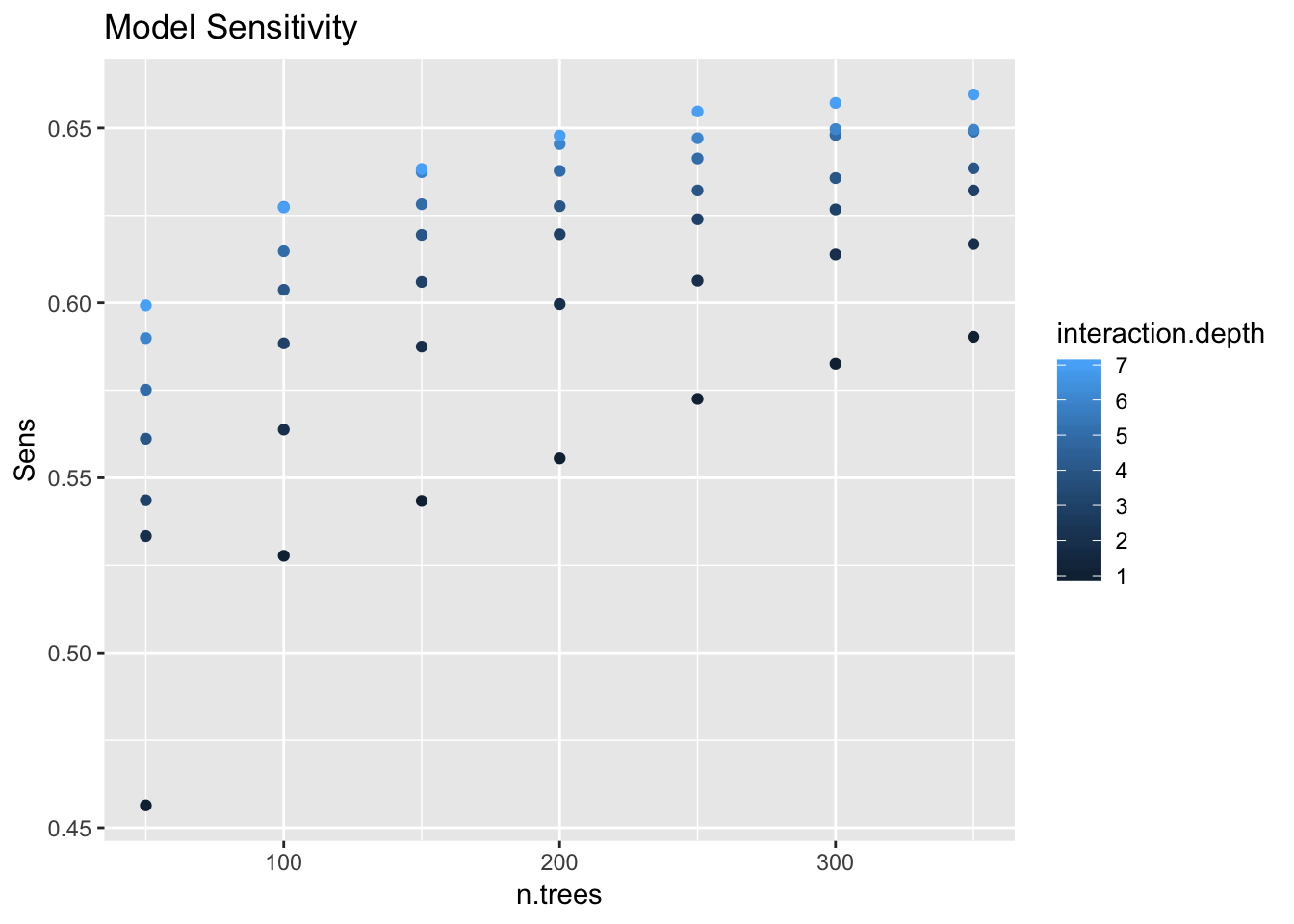

We see a positive trends which stabilizes.

Let us see the metrics on the test set.

pred_df <- get_pred_df(model_obj = gbm_model_2, X_test = X_test, y_test = y_test)
# Confusion Matrix. 
conf_matrix_test <- confusionMatrix(data = pred_df$y_pred, reference =  y_test)
conf_matrix_test

## Confusion Matrix and Statistics
## 
##           Reference
## Prediction large small
##      large  1024   294
##      small   506  4319
##                                           
##                Accuracy : 0.8698          
##                  95% CI : (0.8611, 0.8781)
##     No Information Rate : 0.7509          
##     P-Value [Acc > NIR] : < 2.2e-16       
##                                           
##                   Kappa : 0.6349          
##                                           
##  Mcnemar's Test P-Value : 8.654e-14       
##                                           
##             Sensitivity : 0.6693          
##             Specificity : 0.9363          
##          Pos Pred Value : 0.7769          
##          Neg Pred Value : 0.8951          
##              Prevalence : 0.2491          
##          Detection Rate : 0.1667          
##    Detection Prevalence : 0.2146          
##       Balanced Accuracy : 0.8028          
##                                           
##        'Positive' Class : large           
##

We do not see a significant increase in sensitivity.

pred_df %>% 
  ggplot(mapping = aes(x = y_test, y = y_pred_num, fill = y_test)) +
  geom_boxplot() + 
  geom_abline(slope = 0, 
              intercept = 0.5, 
              alpha = 0.8, 
              linetype = 2, 
              color = "purple4") +
  scale_fill_brewer(palette = "Set1", direction = -1) +
  labs(title = "Preditcted Distributions - GBM Model 2 (Max Sens)", 
       subtitle = "Prediction Cut = 0.5", 
       x = "test label", 
       y = "predicted probability") +
  scale_x_discrete(limits = rev(levels(y_test)))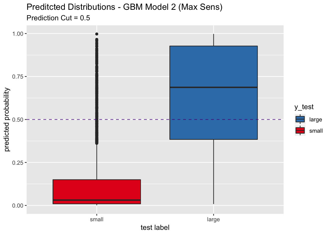

Model Fit - Alternate Cutoffs

We can use the ROC curve to select an alternative cutoff to label the predicted classes Applied Predictive Modeling, Section 16.4. It is important to do this cutoff selection on the evaluation set.

PLS Model

# Parallel Computation.
cl <- makePSOCKcluster(detectCores())
registerDoParallel(cl)

# Train model.
pls_model_3 <- train(x = X_train,
                     y = y_train,
                     method = "pls",
                     family = binomial(link = "logit"), 
                     tuneLength = 10,
                     preProcess = c("scale", "center"), 
                     trControl = train_control,
                     metric = "ROC", 
                     verbose = FALSE)

stopCluster(cl)

model_list$models$pls_model_3 = pls_model_3

Let us see the metrics and ROC curve of the evaluation set:

y_pred_eval <- predict(object = pls_model_3, newdata = X_eval, type = "prob") %>% 
  pull(large) %>% 
  # If the probability is larger than 0.5 we predict large. 
  map_chr(.f = ~ ifelse(test = .x > 0.5, yes = "large", no = "small")) %>% 
  as_factor()

# Confusion Matrix. 
conf_matrix_eval <- confusionMatrix(data = y_pred_eval, reference =  y_eval)
conf_matrix_eval

## Confusion Matrix and Statistics
## 
##           Reference
## Prediction large small
##      large   430   147
##      small   335  2160
##                                           
##                Accuracy : 0.8431          
##                  95% CI : (0.8297, 0.8558)
##     No Information Rate : 0.751           
##     P-Value [Acc > NIR] : < 2.2e-16       
##                                           
##                   Kappa : 0.543           
##                                           
##  Mcnemar's Test P-Value : < 2.2e-16       
##                                           
##             Sensitivity : 0.5621          
##             Specificity : 0.9363          
##          Pos Pred Value : 0.7452          
##          Neg Pred Value : 0.8657          
##              Prevalence : 0.2490          
##          Detection Rate : 0.1400          
##    Detection Prevalence : 0.1878          
##       Balanced Accuracy : 0.7492          
##                                           
##        'Positive' Class : large           
##

y_pred_eval_num <- predict(object = pls_model_3, newdata = X_eval, type = "prob") %>% pull(large)
  
roc_curve_eval <- roc(response = y_eval, 
                      predictor = y_pred_eval_num,
                      levels = c("small", "large"))

auc_pls <- roc_curve_eval %>% 
  auc() %>% 
  round(digits = 3)

plot(roc_curve_eval)
title(main = str_c("PLS Model 3 - ROC AUC (Eval) = ", auc_pls), line = 2.5)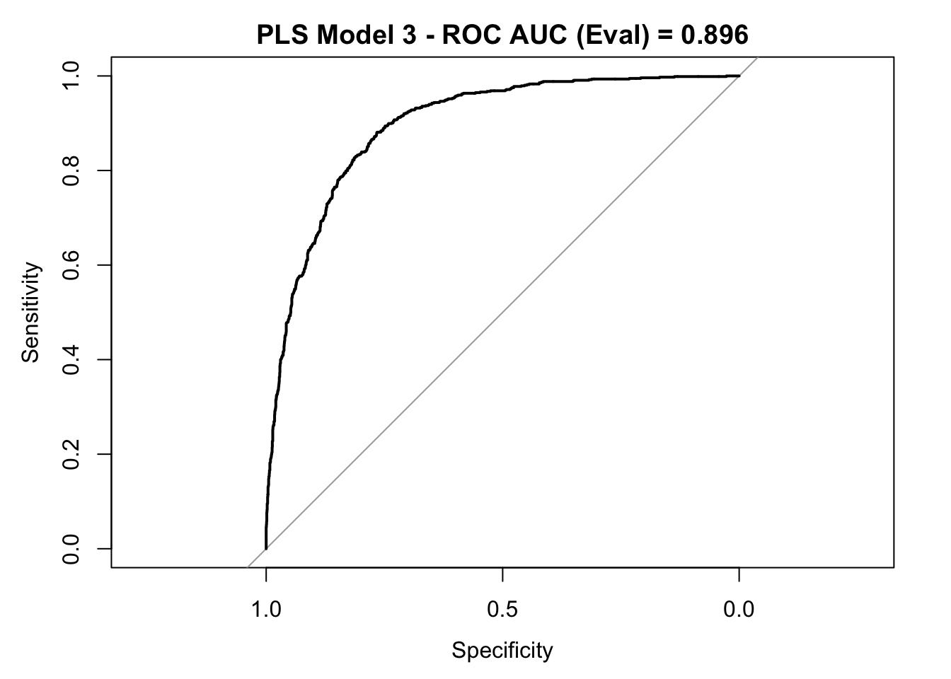

We can use the ROC curve to select the most appropiate prediction cutoff. Depending on the specific prediction problem, one could try to find a balance between sensitivity and specificity. One possibility is to choose the closest point of the ROC curve to the to the upper left corner.

best_point_eval <- coords(
  roc = roc_curve_eval, x = "best", 
   best.method = "closest.topleft"
)

model_list$best_point <- list(pls_model_3 = best_point_eval)

best_point_eval

##   threshold specificity sensitivity 
##   0.4141877   0.8131773   0.8274510

# Get points to plot the ROC curve. 
all_roc_coords <- coords(roc = roc_curve_eval, x = "all", as.list = FALSE)

all_roc_cords_df <- all_roc_coords %>% 
  t() %>%  
  as_tibble()

all_roc_cords_df %>% 
  ggplot() +
  geom_line(mapping = aes(x = 1 - specificity, y = sensitivity)) +
  geom_abline(slope = 1, intercept = 0, linetype = 2) +
  geom_point(mapping = aes(x = (1- best_point_eval[["specificity"]]), 
                           y =  best_point_eval[["sensitivity"]], 
                           color = "optimal point"), 
             
             size = 4) +
  geom_point(mapping = aes(x = (1 - conf_matrix_eval$byClass[["Specificity"]]), 
                           y = conf_matrix_eval$byClass[["Sensitivity"]], 
                           color = "initial cutoff"),
             size = 4) +
  labs(title = "PLS Model 3 - ROC Curve (Eval)")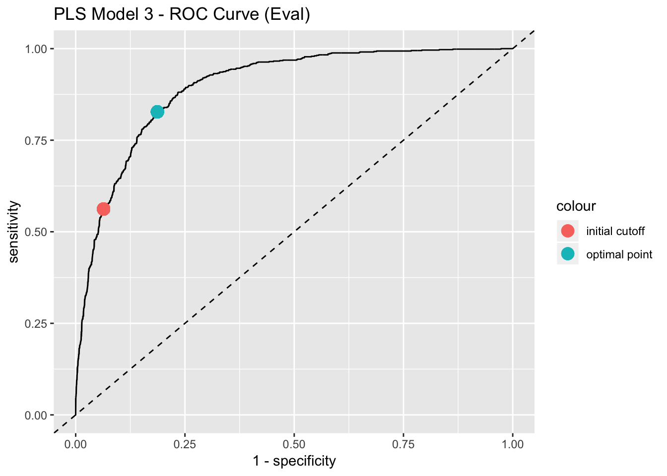

Let us now evaluate the model predictions with this new cutoff point on the test set:

pred_df <- get_pred_df(model_obj = pls_model_3, 
                       X = X_test, 
                       y_test = y_test, 
                       threshold = best_point_eval["threshold"])

pred_df %>% 
  ggplot(mapping = aes(x = y_test, y = y_pred_num, fill = y_test)) +
  geom_boxplot() + 
  geom_abline(slope = 0, 
              intercept = 0.5,
              alpha = 0.8, 
              linetype = 2, 
              color = "purple4") +
  geom_abline(slope = 0, 
              intercept = best_point_eval["threshold"], 
              linetype = 2, 
              color = "dark green") +
  scale_fill_brewer(palette = "Set1", direction = -1) +
  labs(title = "Preditcted Distributions - PLS Model 3 (New Cutoff)", 
       subtitle = str_c("Prediction Cut = ", round(best_point_eval["threshold"], 3)), 
       x = "test label", 
       y = "predicted probability") +
  scale_x_discrete(limits = rev(levels(y_test)))

conf_matrix_test <- confusionMatrix(data = pred_df$y_pred, reference =  y_test)
conf_matrix_test

## Confusion Matrix and Statistics
## 
##           Reference
## Prediction large small
##      large  1254   953
##      small   276  3660
##                                           
##                Accuracy : 0.7999          
##                  95% CI : (0.7897, 0.8099)
##     No Information Rate : 0.7509          
##     P-Value [Acc > NIR] : < 2.2e-16       
##                                           
##                   Kappa : 0.5341          
##                                           
##  Mcnemar's Test P-Value : < 2.2e-16       
##                                           
##             Sensitivity : 0.8196          
##             Specificity : 0.7934          
##          Pos Pred Value : 0.5682          
##          Neg Pred Value : 0.9299          
##              Prevalence : 0.2491          
##          Detection Rate : 0.2041          
##    Detection Prevalence : 0.3593          
##       Balanced Accuracy : 0.8065          
##                                           
##        'Positive' Class : large           
##

We indeed see that the sensitivity increases to around 0.8 on the test set. The trade-off is a decrease in specificity.

GBM Model

# Parallel Computation.
cl <- makePSOCKcluster(detectCores())
registerDoParallel(cl)

# Train model.
gbm_model_3 <- train(x = X_train,
                     y = y_train,
                     method = "gbm",
                     tuneLength = 7,
                     trControl = train_control,
                     metric = "ROC", 
                     verbose = FALSE)

stopCluster(cl)

model_list$models$gbm_model_3 = gbm_model_3

Let us see the metrics and ROC curve of the evaluation set:

y_pred_eval <- predict(object = gbm_model_3, newdata = X_eval, type = "prob") %>% 
  pull(large) %>% 
  # If the probability is larger than 0.5 we predict large. 
  map_chr(.f = ~ ifelse(test = .x > 0.5, yes = "large", no = "small")) %>% 
  as_factor()

# Confusion Matrix. 
conf_matrix_eval <- confusionMatrix(data = y_pred_eval, reference =  y_eval)
conf_matrix_eval

## Confusion Matrix and Statistics
## 
##           Reference
## Prediction large small
##      large   506   145
##      small   259  2162
##                                          
##                Accuracy : 0.8685         
##                  95% CI : (0.856, 0.8802)
##     No Information Rate : 0.751          
##     P-Value [Acc > NIR] : < 2.2e-16      
##                                          
##                   Kappa : 0.63           
##                                          
##  Mcnemar's Test P-Value : 1.888e-08      
##                                          
##             Sensitivity : 0.6614         
##             Specificity : 0.9371         
##          Pos Pred Value : 0.7773         
##          Neg Pred Value : 0.8930         
##              Prevalence : 0.2490         
##          Detection Rate : 0.1647         
##    Detection Prevalence : 0.2119         
##       Balanced Accuracy : 0.7993         
##                                          
##        'Positive' Class : large          
##

y_pred_eval_num <- predict(object = gbm_model_3, newdata = X_eval, type = "prob") %>% pull(large)
  
roc_curve_eval <- roc(response = y_eval, 
                      predictor = y_pred_eval_num,
                      levels = c("small", "large"))

auc_gbm <- roc_curve_eval %>% 
  auc() %>% 
  round(digits = 3)

plot(roc_curve_eval)
title(main = str_c("GBM Model 3 - ROC AUC (Eval) = ", auc_gbm), line = 2.5)

best_point_eval <- coords(
  roc = roc_curve_eval, x = "best", 
   best.method = "closest.topleft"
)

model_list$best_point$gbm_model_3 <- best_point_eval

best_point_eval

##   threshold specificity sensitivity 
##   0.2354104   0.8257477   0.8692810

# Get points to plot the ROC curve. 
all_roc_coords <- coords(roc = roc_curve_eval, x = "all", as.list = FALSE)

all_roc_cords_df <- all_roc_coords %>% 
  t() %>%  
  as_tibble()

all_roc_cords_df %>% 
  ggplot() +
  geom_line(mapping = aes(x = 1- specificity, y = sensitivity)) +
  geom_abline(slope = 1, intercept = 0, linetype = 2) +
  geom_point(mapping = aes(x = (1- best_point_eval[["specificity"]]), 
                           y = best_point_eval[["sensitivity"]], 
                           color = "optimal point"), 
             
             size = 4) +
  geom_point(mapping = aes(x = (1 - conf_matrix_eval$byClass[["Specificity"]]), 
                           y = conf_matrix_eval$byClass[["Sensitivity"]], 
                           color = "initial cutoff"),
             size = 4) +
  labs(title = "GBM Model 3 - ROC Curve (Eval)")

Let us now evaluate the model predictions with this new cutoff point on the test set:

pred_df <- get_pred_df(model_obj = gbm_model_3, 
                       X = X_test, 
                       y_test = y_test, 
                       threshold = best_point_eval["threshold"])

pred_df %>% 
  ggplot(mapping = aes(x = y_test, y = y_pred_num, fill = y_test)) +
  geom_boxplot() + 
  geom_abline(slope = 0, 
              intercept = 0.5,
              alpha = 0.8, 
              linetype = 2, 
              color = "purple4") +
  geom_abline(slope = 0, 
              intercept = best_point_eval["threshold"], 
              linetype = 2, 
              color = "dark green") +
  scale_fill_brewer(palette = "Set1", direction = -1) +
  labs(title = "Preditcted Distributions - GBM Model 3 (New Cutoff)", 
       subtitle = str_c("Prediction Cut = ", round(best_point_eval["threshold"], 3)), 
       x = "test label", 
       y = "predicted probability") +
  scale_x_discrete(limits = rev(levels(y_test)))

conf_matrix_test <- confusionMatrix(data = pred_df$y_pred , reference =  y_test)
conf_matrix_test

## Confusion Matrix and Statistics
## 
##           Reference
## Prediction large small
##      large  1319   796
##      small   211  3817
##                                           
##                Accuracy : 0.8361          
##                  95% CI : (0.8266, 0.8453)
##     No Information Rate : 0.7509          
##     P-Value [Acc > NIR] : < 2.2e-16       
##                                           
##                   Kappa : 0.6114          
##                                           
##  Mcnemar's Test P-Value : < 2.2e-16       
##                                           
##             Sensitivity : 0.8621          
##             Specificity : 0.8274          
##          Pos Pred Value : 0.6236          
##          Neg Pred Value : 0.9476          
##              Prevalence : 0.2491          
##          Detection Rate : 0.2147          
##    Detection Prevalence : 0.3443          
##       Balanced Accuracy : 0.8448          
##                                           
##        'Positive' Class : large           
##

In this case, the sensitivity increases to around 0.86. This model is appropiated if sensitivity is the most relevant metric for the application.

Sampling Methods

Next, we explore sampling methods. The aim is to balance the class frequency in the training set itself Applied Predictive Modeling, Section 16.7.

Up-sampling is any technique that simulates or imputes additional data points to improve balance across classes.
Down-sampling is any technique that reduces the number of samples to improve the balance across classes.

We explore the effect of up-sampling.

Up Sampling

# Generate new training set. 
df_upSample_train <- upSample(x = X_train, 
                             y = y_train, 
                             yname = "income")

X_upSample_train <- df_upSample_train %>% select(- income) 
y_upSample_train <- df_upSample_train %>% pull(income) 

# Get new training data dimension. 
dim(df_upSample_train)

## [1] 32296    47

Let us see the class count:

table(df_upSample_train$income)

## 
## large small 
## 16148 16148

Now we train the models on this new training data.

PLS Model

# Parallel Computation.
cl <- makePSOCKcluster(detectCores())
registerDoParallel(cl)

# Train model.
pls_model_4 <- train(x = X_upSample_train,
                     y = y_upSample_train,
                     method = "pls",
                     family = binomial(link = "logit"), 
                     tuneLength = 10,
                     preProcess = c("scale", "center"), 
                     trControl = train_control,
                     metric = "ROC", 
                     verbose = FALSE)

stopCluster(cl)

model_list$models$pls_model_4 = pls_model_4

pred_df <- get_pred_df(model_obj = pls_model_4, X = X_test, y_test = y_test)
# Confusion Matrix. 
conf_matrix_test <- confusionMatrix(data = pred_df$y_pred, reference =  y_test)
conf_matrix_test

## Confusion Matrix and Statistics
## 
##           Reference
## Prediction large small
##      large  1307  1062
##      small   223  3551
##                                           
##                Accuracy : 0.7908          
##                  95% CI : (0.7804, 0.8009)
##     No Information Rate : 0.7509          
##     P-Value [Acc > NIR] : 9.847e-14       
##                                           
##                   Kappa : 0.5274          
##                                           
##  Mcnemar's Test P-Value : < 2.2e-16       
##                                           
##             Sensitivity : 0.8542          
##             Specificity : 0.7698          
##          Pos Pred Value : 0.5517          
##          Neg Pred Value : 0.9409          
##              Prevalence : 0.2491          
##          Detection Rate : 0.2128          
##    Detection Prevalence : 0.3856          
##       Balanced Accuracy : 0.8120          
##                                           
##        'Positive' Class : large           
##

For this model, the sensitivity is higher than the one obtained after optimizing the probability cutoff.

pred_df %>% 
  ggplot(mapping = aes(x = y_test, y = y_pred_num, fill = y_test)) +
  geom_boxplot() + 
  geom_abline(slope = 0, 
              intercept = 0.5, 
              alpha = 0.8, 
              linetype = 2, 
              color = "purple4", show.legend = TRUE) +
  scale_fill_brewer(palette = "Set1", direction = -1) +
  labs(title = "Preditcted Distributions - PLS Model 4 (Up Sampling)", 
       subtitle = "Prediction Cut = 0.5", 
       x = "test label", 
       y = "predicted probability") +
  scale_x_discrete(limits = rev(levels(y_test)))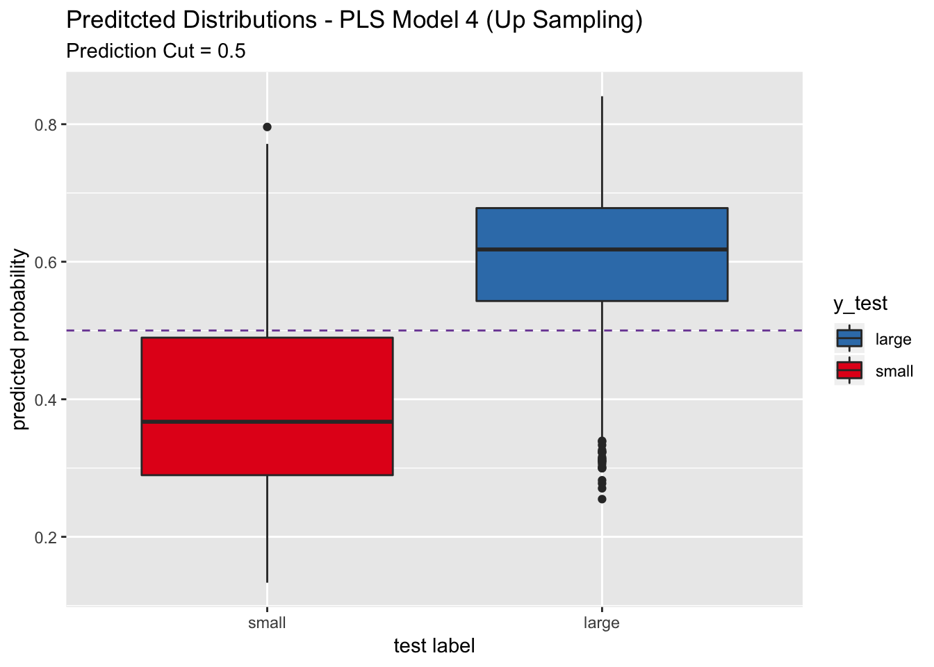

roc_curve_test <- roc(response = y_test, 
                      pred_df$y_pred_num, 
                      levels = c("small", "large"))

auc_pls <- roc_curve_test %>% 
  auc() %>% 
  round(digits = 3)

plot(roc_curve_test)
title(main = str_c("PLS Model 4 - ROC AUC (Test) = ", auc_pls), line = 2.5)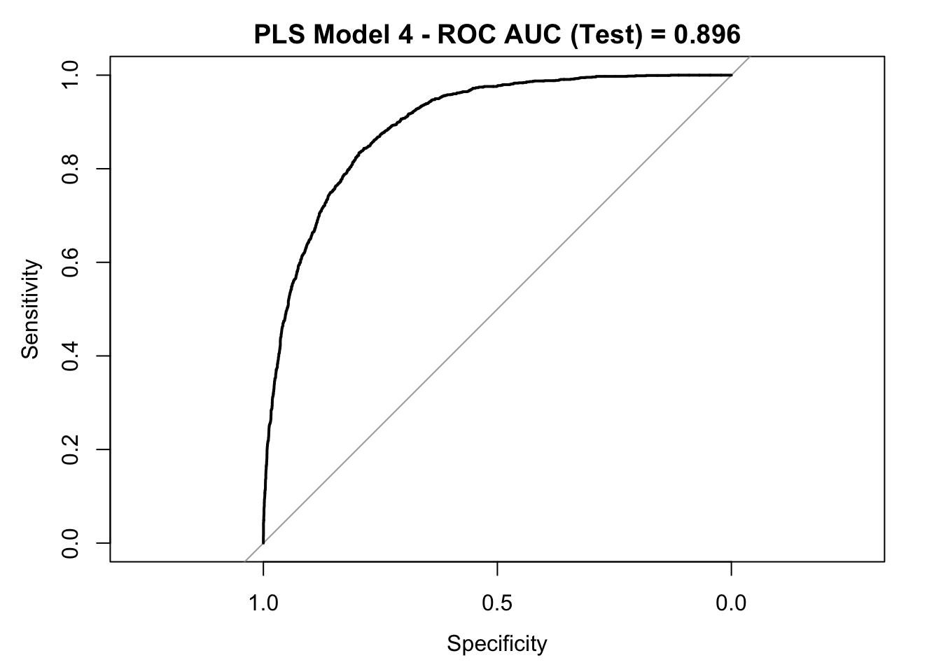

GBM Model

# Parallel Computation.
cl <- makePSOCKcluster(detectCores())
registerDoParallel(cl)

# Train model.
gbm_model_4 <- train(x = X_upSample_train,
                     y = y_upSample_train,
                     method = "gbm",
                     tuneLength = 7,
                     trControl = train_control,
                     metric = "ROC", 
                     verbose = FALSE)

stopCluster(cl)

model_list$models$gbm_model_4 = gbm_model_4

pred_df <- get_pred_df(model_obj = gbm_model_4 , X = X_test, y_test = y_test)
# Confusion Matrix. 
conf_matrix_test <- confusionMatrix(data = pred_df$y_pred, reference =  y_test)
conf_matrix_test

## Confusion Matrix and Statistics
## 
##           Reference
## Prediction large small
##      large  1306   750
##      small   224  3863
##                                           
##                Accuracy : 0.8414          
##                  95% CI : (0.8321, 0.8505)
##     No Information Rate : 0.7509          
##     P-Value [Acc > NIR] : < 2.2e-16       
##                                           
##                   Kappa : 0.6198          
##                                           
##  Mcnemar's Test P-Value : < 2.2e-16       
##                                           
##             Sensitivity : 0.8536          
##             Specificity : 0.8374          
##          Pos Pred Value : 0.6352          
##          Neg Pred Value : 0.9452          
##              Prevalence : 0.2491          
##          Detection Rate : 0.2126          
##    Detection Prevalence : 0.3347          
##       Balanced Accuracy : 0.8455          
##                                           
##        'Positive' Class : large           
##

pred_df %>% 
  ggplot(mapping = aes(x = y_test, y = y_pred_num, fill = y_test)) +
  geom_boxplot() + 
  geom_abline(slope = 0, 
              intercept = 0.5, 
              alpha = 0.8, 
              linetype = 2, 
              color = "purple4", show.legend = TRUE) +
  scale_fill_brewer(palette = "Set1", direction = -1) +
  labs(title = "Preditcted Distributions - GBM Model 4 (Up Sampling)", 
       subtitle = "Prediction Cut = 0.5", 
       x = "test label", 
       y = "predicted probability") +
  scale_x_discrete(limits = rev(levels(y_test)))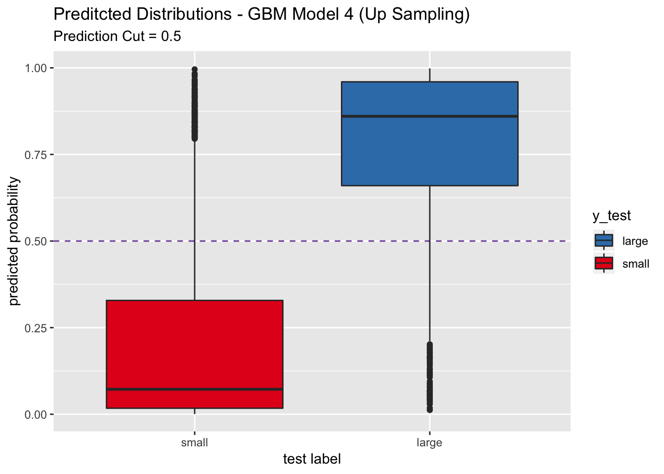

roc_curve_test <- roc(response = y_test, 
                      pred_df$y_pred_num, 
                      levels = c("small", "large"))

auc_gbm <- roc_curve_test %>% 
  auc() %>% 
  round(digits = 3)

plot(roc_curve_test)
title(main = str_c("GBM Model 4 - ROC AUC (Test) = ", auc_gbm), line = 2.5)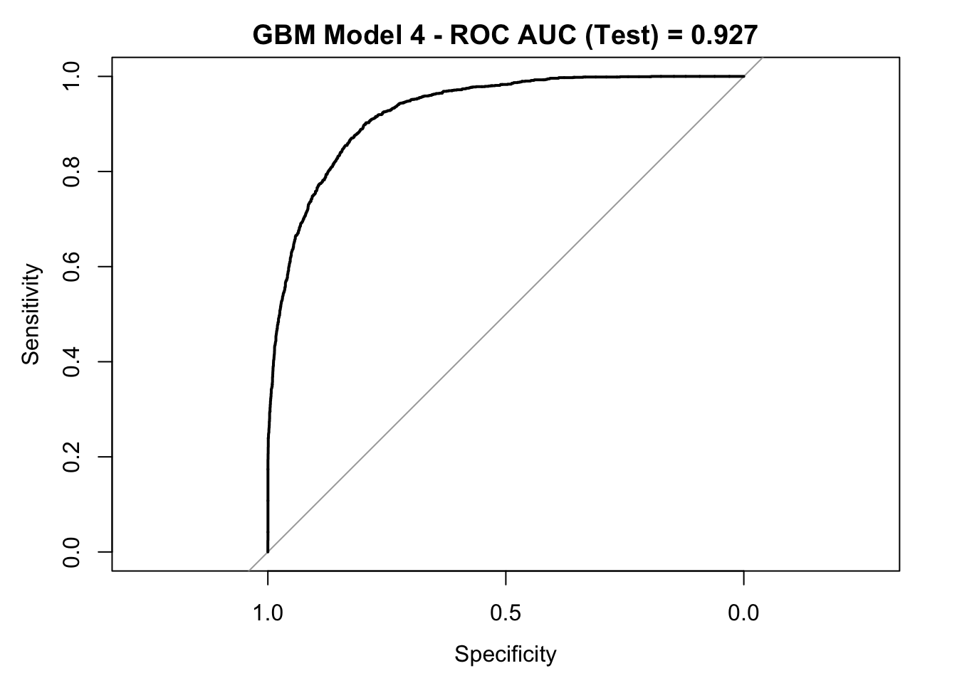

Warning: “When using modified versions of the training set, resampled estimates of model performance can become biased. For example, if the data are up-sampled, resampling procedures are likely to have the same sample in the cases that are used to build the model as well as the holdout set, leading to optimistic results. Despite this, resampling methods can still be effective at tuning the models”.

SMOTE

“The synthetic minority over-sampling technique (SMOTE) is a data sampling procedure that uses both up-sampling and down-sampling, depending on the class, and has three operational paameters: the amount of up-sampling, the amount of down-sampling, and the number of neighbors that are used to impute new cases. To up-sample for the minority class, SMOTE synthesizes new cases. To do this, a data point is randomly selected from the minority class and its K-nearest neighbors are determined”. Applied Predictive Modeling, Section 16.7

# Get new training set.
df_smote_train <-  DMwR::SMOTE(
  form = income ~ .,
  perc.over = 200, 
  perc.under = 150, 
  data = as.data.frame(bind_cols(income = y_train, X_train))
)

X_smote_train <- df_smote_train  %>% select(- income) 
y_smote_train <- df_smote_train  %>% pull(income) 

# Get new training data dimension. 
dim(df_smote_train)

## [1] 32130    47

table(df_smote_train$income)

## 
## large small 
## 16065 16065

PLS Model

# Parallel Computation.
cl <- makePSOCKcluster(detectCores())
registerDoParallel(cl)

# Train model.
pls_model_5 <- train(x = X_smote_train,
                     y = y_smote_train,
                     method = "pls",
                     family = binomial(link = "logit"), 
                     tuneLength = 10,
                     preProcess = c("scale", "center"), 
                     trControl = train_control,
                     metric = "ROC", 
                     verbose = FALSE)

stopCluster(cl)

model_list$models$pls_model_5 = pls_model_5

pred_df <- get_pred_df(model_obj = pls_model_5 , X = X_test, y_test = y_test)
# Confusion Matrix. 
conf_matrix_test <- confusionMatrix(data = pred_df$y_pred, reference =  y_test)
conf_matrix_test

## Confusion Matrix and Statistics
## 
##           Reference
## Prediction large small
##      large  1184   889
##      small   346  3724
##                                           
##                Accuracy : 0.799           
##                  95% CI : (0.7887, 0.8089)
##     No Information Rate : 0.7509          
##     P-Value [Acc > NIR] : < 2.2e-16       
##                                           
##                   Kappa : 0.5195          
##                                           
##  Mcnemar's Test P-Value : < 2.2e-16       
##                                           
##             Sensitivity : 0.7739          
##             Specificity : 0.8073          
##          Pos Pred Value : 0.5712          
##          Neg Pred Value : 0.9150          
##              Prevalence : 0.2491          
##          Detection Rate : 0.1927          
##    Detection Prevalence : 0.3375          
##       Balanced Accuracy : 0.7906          
##                                           
##        'Positive' Class : large           
##

pred_df %>% 
  ggplot(mapping = aes(x = y_test, y = y_pred_num, fill = y_test)) +
  geom_boxplot() + 
  geom_abline(slope = 0, 
              intercept = 0.5, 
              alpha = 0.8, 
              linetype = 2, 
              color = "purple4", show.legend = TRUE) +
  scale_fill_brewer(palette = "Set1", direction = -1) +
  labs(title = "Preditcted Distributions - PLS Model 5 (SMOTE)", 
       subtitle = "Prediction Cut = 0.5", 
       x = "test label", 
       y = "predicted probability") +
  scale_x_discrete(limits = rev(levels(y_test)))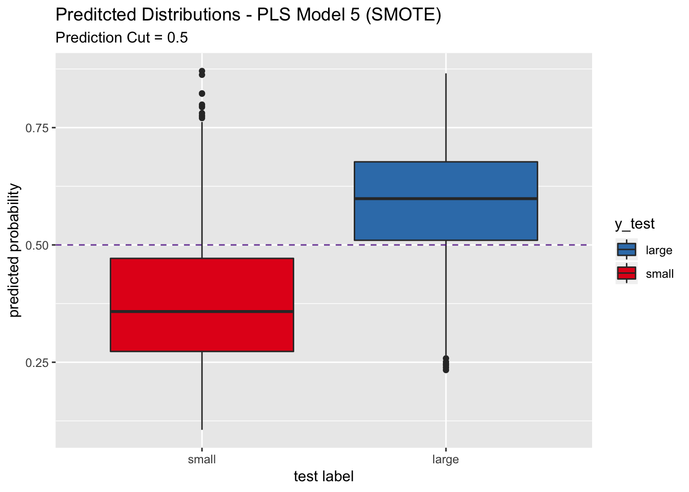

roc_curve_test <- roc(response = y_test, 
                      pred_df$y_pred_num, 
                      levels = c("small", "large"))

auc_pls <- roc_curve_test %>% 
  auc() %>% 
  round(digits = 3)

plot(roc_curve_test)
title(main = str_c("PLS Model 5 - ROC AUC (Test) = ", auc_pls), line = 2.5)

GBM Model

# Parallel Computation.
cl <- makePSOCKcluster(detectCores())
registerDoParallel(cl)

# Train model.
gbm_model_5 <- train(x = X_smote_train,
                     y = y_smote_train,
                     method = "gbm",
                     tuneLength = 7,
                     trControl = train_control,
                     metric = "ROC", 
                     verbose = FALSE)

stopCluster(cl)

model_list$models$gbm_model_5 = gbm_model_5

pred_df <- get_pred_df(model_obj = gbm_model_5 , X = X_test, y_test = y_test)
# Confusion Matrix. 
conf_matrix_test <- confusionMatrix(data = pred_df$y_pred, reference =  y_test)
conf_matrix_test

## Confusion Matrix and Statistics
## 
##           Reference
## Prediction large small
##      large  1038   345
##      small   492  4268
##                                           
##                Accuracy : 0.8637          
##                  95% CI : (0.8549, 0.8722)
##     No Information Rate : 0.7509          
##     P-Value [Acc > NIR] : < 2e-16         
##                                           
##                   Kappa : 0.6237          
##                                           
##  Mcnemar's Test P-Value : 4.5e-07         
##                                           
##             Sensitivity : 0.6784          
##             Specificity : 0.9252          
##          Pos Pred Value : 0.7505          
##          Neg Pred Value : 0.8966          
##              Prevalence : 0.2491          
##          Detection Rate : 0.1690          
##    Detection Prevalence : 0.2251          
##       Balanced Accuracy : 0.8018          
##                                           
##        'Positive' Class : large           
##

pred_df %>% 
  ggplot(mapping = aes(x = y_test, y = y_pred_num, fill = y_test)) +
  geom_boxplot() + 
  geom_abline(slope = 0, 
              intercept = 0.5, 
              alpha = 0.8, 
              linetype = 2, 
              color = "purple4", show.legend = TRUE) +
  scale_fill_brewer(palette = "Set1", direction = -1) +
  labs(title = "Preditcted Distributions - GBM Model 5 (SMOTE)", 
       subtitle = "Prediction Cut = 0.5", 
       x = "test label", 
       y = "predicted probability") +
  scale_x_discrete(limits = rev(levels(y_test)))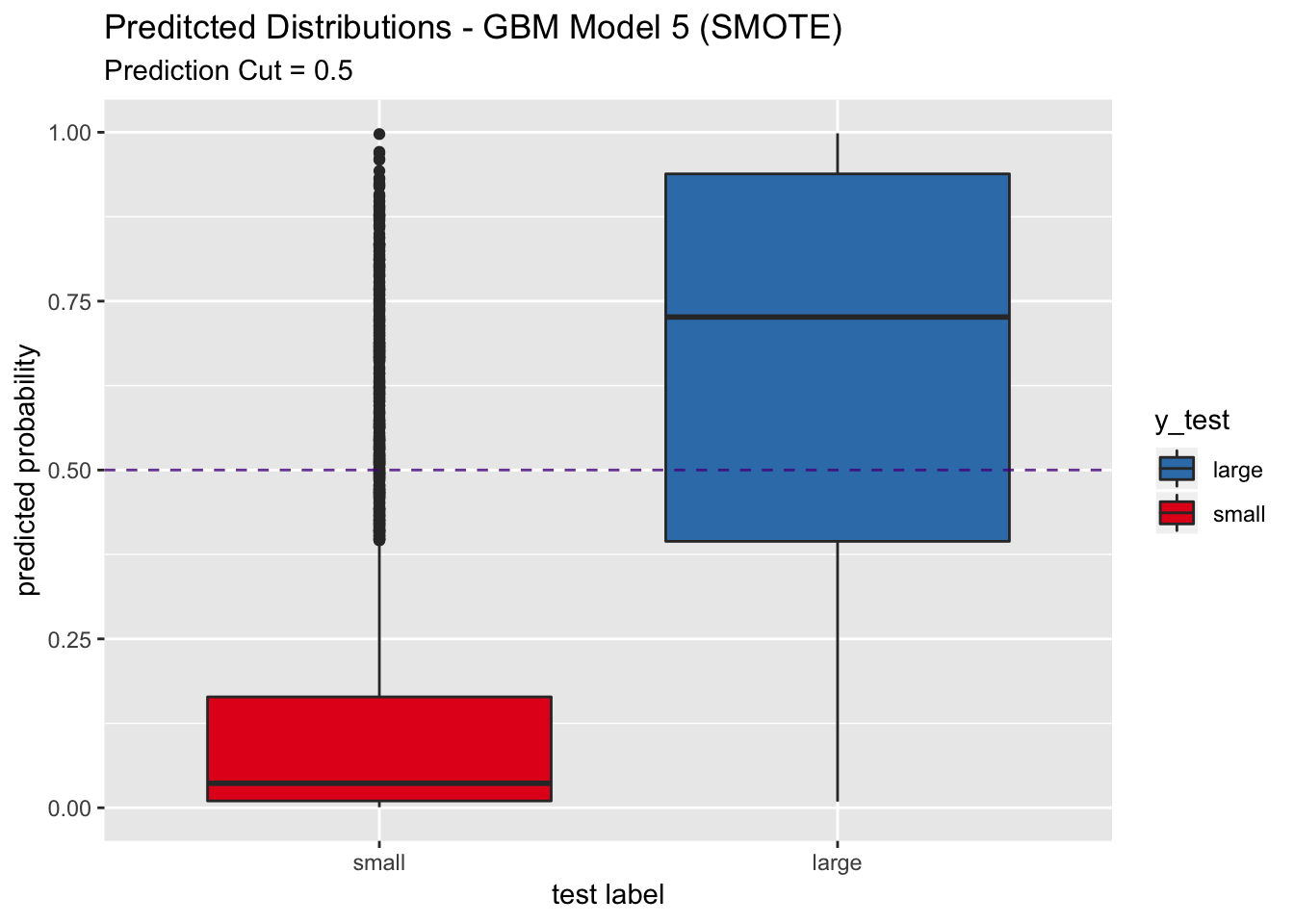

roc_curve_test <- roc(response = y_test, 
                      pred_df$y_pred_num, 
                      levels = c("small", "large"))

auc_gbm <- roc_curve_test %>% 
  auc() %>% 
  round(digits = 3)

plot(roc_curve_test)
title(main = str_c("GBM Model 5 - ROC AUC (Test) = ", auc_gbm), line = 2.5)

Model Summary

Let us parse the model results.

generate_model_summary <- function (model_lis) {
  
  models_summary <- names(model_list$models) %>% 
    
    map_df(.f = function(m_name) {
      
      m <- model_list$models[[m_name]]
      
      m_threshold <- 0.5
      
      if (m_name %in% names(model_list$best_point)) {
        
        m_threshold <- model_list$best_point[[m_name]][["threshold"]]
        
      }
      
      y_pred <- predict(object = m , newdata = X_test, type = "prob") %>% 
        pull(large) %>% 
        # If the probability is larger than 0.5 we predict large. 
        map_chr(.f = ~ ifelse(test = .x > m_threshold, yes = "large", no = "small")) %>% 
        as_factor()
    
      # Confusion Matrix. 
      conf_matrix_test <- confusionMatrix(data = y_pred, reference =  y_test)
      
      conf_matrix_test$byClass %>% 
        t() %>% 
        as_tibble() %>% 
        select(Sensitivity, Specificity, Precision, Recall, F1) 
    }
  )

  models_summary %<>% 
    add_column(Model = names(model_list$models), .before = "Sensitivity") %>% 
    separate(col = Model, into = c("Method", "Model", "Tag"), sep = "_") %>% 
    select(- Model) %>% 
    mutate(
      Tag = case_when(
        Tag == 1 ~ "Accuracy", 
        Tag == 2 ~ "Sens", 
        Tag == 3 ~ "Alt Cutoff", 
        Tag == 4 ~ "Up Sampling", 
        Tag == 5 ~ "SMOTE", 
      )
    ) 

  models_summary %<>% mutate_if(.predicate = is.numeric, .funs = ~ round(x = .x, digits = 3))
  
  return(models_summary)
}

models_summary <- generate_model_summary(model_lis = model_list)

models_summary %>% knitr::kable(align = rep("c", 7))

Method	Tag	Sensitivity	Specificity	Precision	Recall	F1
pls	Accuracy	0.552	0.932	0.730	0.552	0.628
gbm	Accuracy	0.655	0.940	0.782	0.655	0.713
pls	Sens	0.561	0.932	0.733	0.561	0.636
gbm	Sens	0.669	0.936	0.777	0.669	0.719
pls	Alt Cutoff	0.820	0.793	0.568	0.820	0.671
gbm	Alt Cutoff	0.862	0.827	0.624	0.862	0.724
pls	Up Sampling	0.854	0.770	0.552	0.854	0.670
gbm	Up Sampling	0.854	0.837	0.635	0.854	0.728
pls	SMOTE	0.774	0.807	0.571	0.774	0.657
gbm	SMOTE	0.678	0.925	0.751	0.678	0.713

# Save Model List. 
saveRDS(object = model_list, file = "model_list.rds")

satRday Berlin 2019: Remedies for Severe Class Imbalance