Prepare the Notebook

library(tidyverse)

Generate Circle Data

# Dimension of the space.
d <- 2

# Number of sample points. 
N <- 1000

# Radius. 
R <- 4

# Generate random sample of points (x - axis).
points.0 <- 1:N %>% map(.f = ~ runif(n = d - 1, min =  - R, max = R))

# Generate the corresponding y - coordinates. 
all.points <- points.0 %>% map(.f = ~ c(., sign(runif(n = 1, min = - 1, max = 1))*sqrt(R^2 - norm(., type = '2')^2))) 

# Store data in a tibble.
all.points.df <- all.points %>% reduce(.f = ~ rbind(.x, .y)) %>% 
                                as.tibble %>% 
                                rename(x = V1, y = V2)

# Plot the data. 
all.points.df %>% 
  ggplot() + 
  theme_light() + 
  geom_point(mapping = aes(x = x, y = y))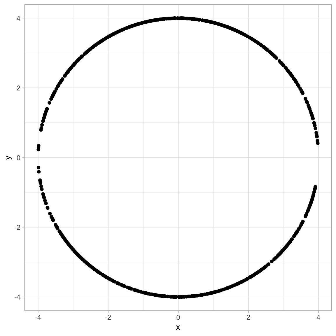 

Add Noise

We add noise from a normal disttribution with mean zero and standard deviation sd.

# Set standard deviation.
sd <- 0.5

# Add noise.
all.samples <- all.points %>% map(.f =  ~ . + rnorm(n = d, mean = 0, sd = sd))

# Store data in a tibble.
all.samples.df <- all.samples %>% reduce(.f = ~ rbind(.x, .y)) %>%
                                  as.tibble %>% 
                                  rename(x = V1, y = V2)

# Plot the data.
all.samples.df %>% 
  ggplot() + 
  theme_light() +
  geom_point(mapping = aes(x = x, y = y))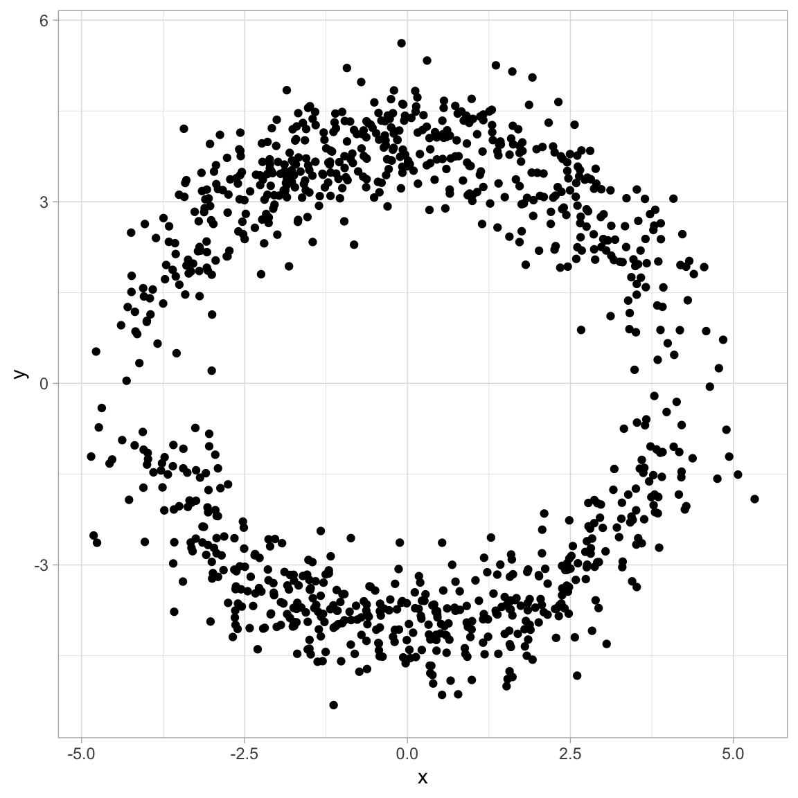 

Define Optimization Function

In order to find the best fitting circle, we need to define what “best” means. We aim to minimize the RMSE.

# Define function to optimize. 
ComputeRMSE <- function(all.samples, r, N) {
  
  all.samples %>% map_dbl(.f = ~ (r - norm(., type = '2'))^2) %>% mean
  
}

Let us visualize the shape of the cost function.

rmse.df <- seq(from = 0.5, to = 10, by = 0.1) %>% 
              map(.f = ~ c(., ComputeRMSE(all.samples = all.samples, r = ., N = N ))) %>% 
              reduce(.f = ~ rbind(.x, .y)) %>% 
              as.tibble %>% 
              rename(r = V1, RMSE = V2)

rmse.df %>% 
  ggplot() + 
  theme_light() + 
  geom_line(mapping = aes(x = r, y = RMSE))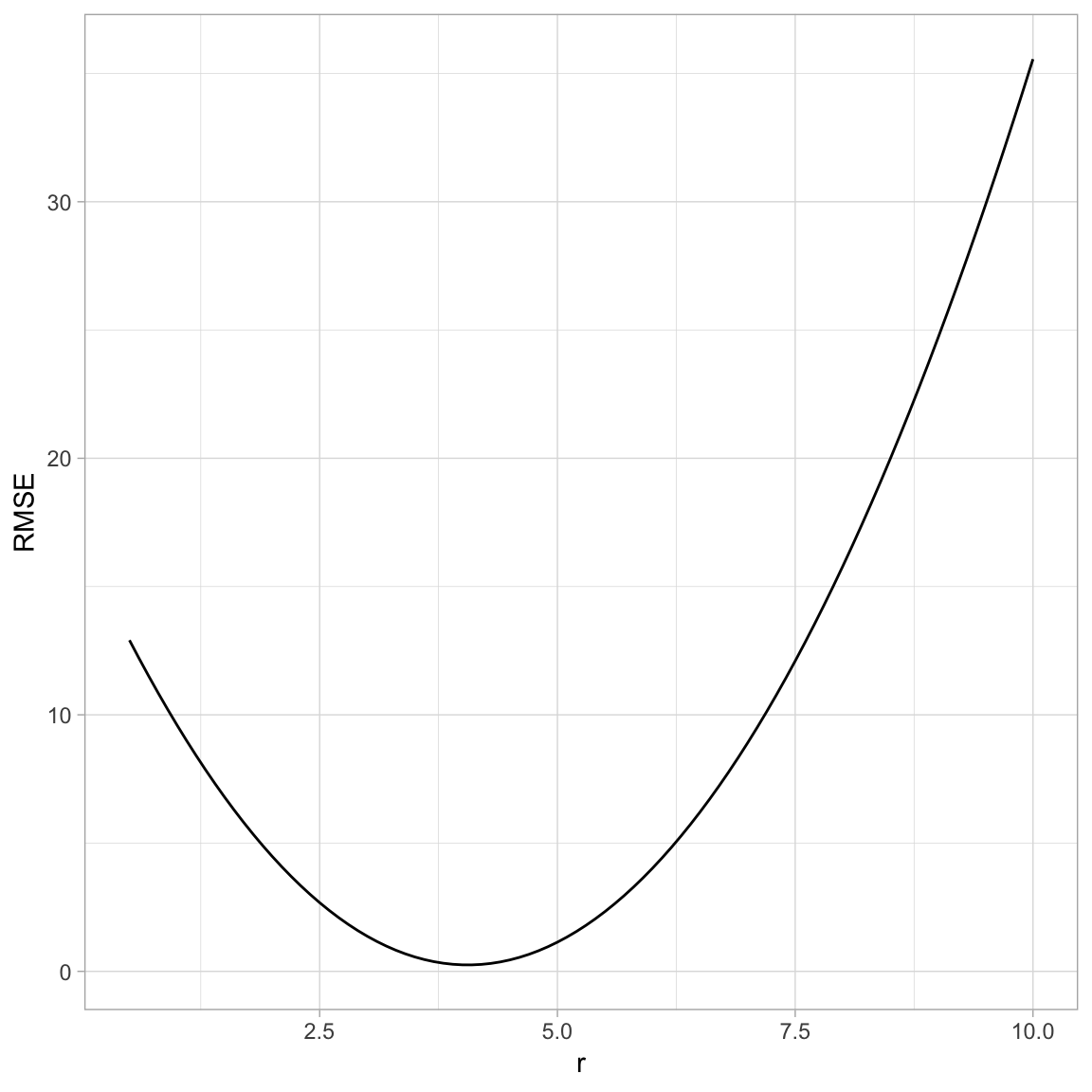

We aim to find the minimum.

Run Optimization

opt.obj <- optimize(f = function(r) ComputeRMSE(all.samples = all.samples, r = r, N = N), 
                    interval = 1:10)

r.hat <- opt.obj$minimum

r.hat

## [1] 4.057873

Visualize Results

We project each sample point onto the best circle fit.

all.samples %>% map(.f = function(x) r.hat*x /norm(x, type = '2')) %>% 
                reduce(.f = function(x, y) rbind(x, y)) %>% 
                as.tibble %>% 
                rename(x1 = V1, y1 =V2) %>% 
                cbind(all.samples.df) %>% 
                ggplot() + 
                theme_light() + 
                geom_point(mapping = aes(x = x, y = y)) +
                geom_point(mapping = aes(x = x1, y = y1), color = 'red')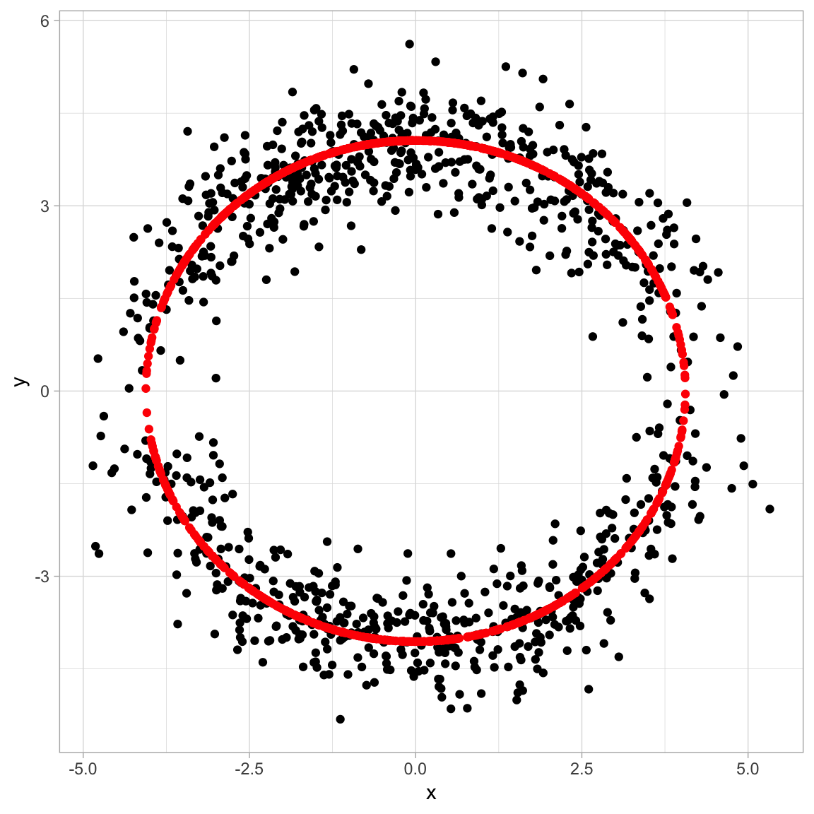 

Analytical Solution

By taking the derivative of the cost function with respect to r we can easily get the value of r.hat.

r.hat <- all.samples %>% map_dbl(.f = ~ norm(., type = '2')) %>% mean

r.hat

## [1] 4.057873