Estimating causal effects from clustered or grouped data requires careful attention to the hierarchical structure of observations. When units are nested within groups such as students within classrooms, or patients within hospitals—ignoring this structure can lead to incorrect standard errors, inefficient estimates, and invalid causal inferences. Multilevel models provide a principled framework for handling such data while leveraging the advantages of partial pooling across groups.
This notebook reproduces and extends the analysis from Chapter 23 of Gelman and Hill’s “Data Analysis Using Regression and Multilevel/Hierarchical Models”. We demonstrate two complementary approaches to modeling treatment effects in hierarchical data: first, a model with varying intercepts that efficiently controls for group-level confounding, and second, a more flexible covariance model that allows treatment effects themselves to vary across groups. Together, these models illustrate how multilevel structures enhance both the efficiency and interpretability of causal effect estimation. In addition to reproducing the analysis, we show how to efficiently vectorize the model (across grades and pairs) using PyMC.
Remark: This example is also treated in ChiRho’s example notebook structured latent confounders.
Context
In the 1970s, an educational television show called “The Electric Company” was produced to help children learn to read. A randomized experiment was conducted to estimate the causal effect of watching the show on reading test scores. This study provides an excellent setting for demonstrating multilevel modeling techniques in causal inference, as the experimental design naturally produces clustered data.
Study Design
The experiment employed a paired randomized design across schools and grades:
Pairs: Classrooms were matched into pairs within the same school and grade (e.g., two 1st grade classes in the same school).
Treatment: Within each pair, one classroom was randomly assigned to the treatment group (watched the show regularly) and the other to the control group (did not watch).
Outcome: Reading test scores at the end of the academic year (
post_test), with adjustment for pre-test scores (pre_test) to increase precision.
This paired randomized design is powerful because randomization within pairs ensures that treatment assignment is independent of pair-level confounders such as school quality, neighborhood characteristics, and baseline achievement levels. However, even though treatment assignment is randomized, the data structure is inherently clustered: students within the same pair (same school and grade) share common characteristics and are therefore correlated in their outcomes. This clustering means that observations within a pair are not statistically independent and they tend to be more similar to each other than to observations from other pairs. Multilevel models are essential here: they correctly account for this within-pair correlation in the outcome variable, leading to valid standard errors and efficient estimates of both average treatment effects and the heterogeneity of effects across pairs.
Outline
We proceed in two parts:
Part 1: We estimate a Hierarchical Intercept Model where pair-specific intercepts account for baseline differences across groups while assuming a common treatment effect. In this example, we also compare two ways to compute the average treatment effect: via direct parameter estimation and via the
marginaleffectspackage and PyMCdooperator to generate counterfactual predictions.Part 2: We extend to a Covariance Model that allows both intercepts and treatment effects to vary across pairs, capturing treatment effect heterogeneity and estimating the correlation between baseline performance and treatment response.
Part 1: Hierarchical Intercept Model
Prepare Notebook
We begin by importing the necessary libraries.
import arviz as az
import matplotlib.pyplot as plt
import numpy as np
import polars as pl
import preliz as pz
import pymc as pm
import pytensor.tensor as pt
import seaborn as sns
from marginaleffects import datagrid
from sklearn.compose import ColumnTransformer
from sklearn.preprocessing import OrdinalEncoder, StandardScaler

az.style.use("arviz-darkgrid")
plt.rcParams["figure.figsize"] = [10, 6]
plt.rcParams["figure.dpi"] = 100
plt.rcParams["figure.facecolor"] = "white"

%load_ext autoreload
%autoreload 2
%config InlineBackend.figure_format = "retina"
seed: int = sum(map(ord, "bayes"))
rng: np.random.Generator = np.random.default_rng(seed=seed)Read Data
We load the Electric Company dataset (from Aki Vehtari’s repository). The data contains pre-test and post-test reading scores for students in paired classrooms across four grade levels. Each pair consists of one treatment and one control classroom.
data_path = "https://raw.githubusercontent.com/avehtari/ROS-Examples/master/ElectricCompany/data/electric.csv"
raw_df = pl.read_csv(data_path).drop(["supp", ""]).sort(["grade", "pair_id"])

raw_df.head()| post_test | pre_test | grade | treatment | pair_id |
|---|---|---|---|---|
| f64 | f64 | i64 | i64 | i64 |
| 48.9 | 13.8 | 1 | 1 | 1 |
| 52.3 | 12.3 | 1 | 0 | 1 |
| 70.5 | 16.5 | 1 | 1 | 2 |
| 55.0 | 14.4 | 1 | 0 | 2 |
| 89.7 | 18.5 | 1 | 1 | 3 |
The dataset includes: grade (grade level), pair_id (identifier for matched classroom pairs), treatment (binary indicator), pre_test (baseline reading score), and post_test (outcome reading score).
Exploratory Data Analysis
Before modeling, it is essential to understand the structure and variability in the data. Since the design relies on paired classrooms, we should inspect the distribution of test scores across grades and pairs to identify the sources of variation that our multilevel model must capture.
g = sns.pairplot(
    raw_df.to_pandas(),
    vars=["pre_test", "grade", "post_test"],
    hue="treatment",
    diag_kind="hist",
)
g.figure.suptitle("Pairwise Relationships", fontsize=18, fontweight="bold", y=1.02);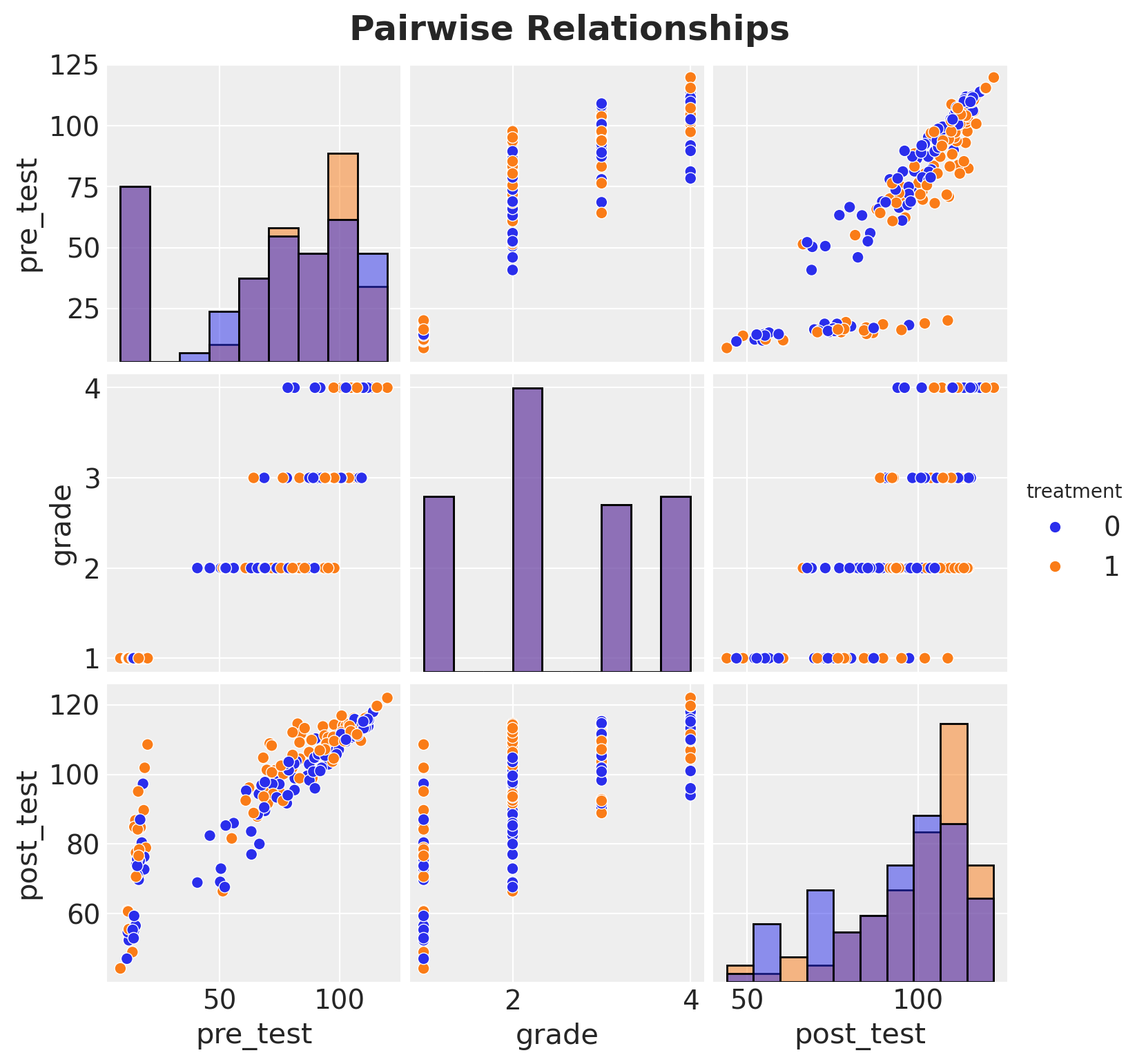
The naive treatment effect is the difference between the mean post-test scores of the treatment and control groups:
(
    raw_df.group_by(["grade", "treatment"])
    .agg(pl.col("post_test").mean())
    .pivot(index="grade", on="treatment", values="post_test")
    .with_columns(pl.col("1").sub(pl.col("0")).alias("treatment_effect"))
    .sort(by="grade")
)| grade | 1 | 0 | treatment_effect |
|---|---|---|---|
| i64 | f64 | f64 | f64 |
| 1 | 77.090476 | 68.790476 | 8.3 |
| 2 | 101.570588 | 93.211765 | 8.358824 |
| 3 | 106.51 | 106.175 | 0.335 |
| 4 | 114.066667 | 110.357143 | 3.709524 |
Data Preprocessing
We standardize the numeric variables (test scores) to facilitate prior specification and improve sampling efficiency. Grade and pair identifiers are encoded as integers for use as group indices in the hierarchical model.
numeric_features = ["pre_test", "post_test"]
ordinal_features = ["grade", "pair_id"]

preprocessor = ColumnTransformer(
    [
        ("num", StandardScaler(), numeric_features),
        ("ord", OrdinalEncoder(dtype=int), ordinal_features),
    ],
    remainder="passthrough",
    verbose_feature_names_out=False,
).set_output(transform="polars")


df = preprocessor.fit_transform(raw_df)

df.head()| pre_test | post_test | grade | pair_id | treatment |
|---|---|---|---|---|
| f64 | f64 | i64 | i64 | i64 |
| -1.726248 | -2.724052 | 0 | 0 | 1 |
| -1.770568 | -2.532096 | 0 | 0 | 0 |
| -1.646472 | -1.504567 | 0 | 1 | 1 |
| -1.70852 | -2.37966 | 0 | 1 | 0 |
| -1.587379 | -0.42058 | 0 | 2 | 1 |
We extract the covariate matrix containing only the pre-test scores, which will be used to control for baseline differences when estimating the treatment effect.
x_columns = ["pre_test"]
x_df = df[x_columns]

x_df.head()| pre_test |
|---|
| f64 |
| -1.726248 |
| -1.770568 |
| -1.646472 |
| -1.70852 |
| -1.587379 |
Next, we set up the coordinate system for our PyMC model. This includes dimensions for covariates, grades, pairs, and observations, which will allow us to structure the hierarchical relationships in the data.
n_grades = len(preprocessor["ord"].categories_[ordinal_features.index("grade")])
n_pairs = len(preprocessor["ord"].categories_[ordinal_features.index("pair_id")])

coords = {
    # covariates
    "covariates": x_df.columns,
    # grade
    "grade": preprocessor["ord"].categories_[ordinal_features.index("grade")],
    # object categories (groups)
    "pair_id": preprocessor["ord"].categories_[ordinal_features.index("pair_id")],
    # index
    "obs_idx": np.arange(len(df)),
}
Model Specification
Motivation: Why Multilevel?
The data is clustered into pairs of classrooms. Observations within the same pair (same school/grade) are likely correlated due to shared unobserved factors like school quality, neighborhood demographics, or teacher characteristics. Ignoring this structure would violate the independence assumption of standard regression.
To estimate the causal effect, we have two main strategies to handle this clustering:
Alternative 1: Fixed Effects (FE)
We could include a dummy variable (intercept) for every pair.
Pros: This controls for ALL time-invariant pair-level unobserved confounders. It effectively “closes back doors” related to the school or neighborhood (see The Effect, Chapter 16).
Cons: It consumes a massive number of degrees of freedom (\(n/2\) parameters just for intercepts!). With many small groups (pairs), this can lead to noisy and inefficient estimates. Of course we could use the Frisch-Waugh-Lovell theorem to demean the data as implemented in the PyFixest package.
Alternative 2: Random Effects (RE) / Hierarchical Intercepts
We model the pair intercepts as coming from a common distribution, e.g., \(\alpha_{j} \sim \text{Normal}(\mu, \sigma)\).
Pros: This uses partial pooling. The model learns the variance \(\sigma\) and “shrinks” noisy pair estimates toward the global mean. It is far more efficient than FE.
Cons: For this we need to expand a bit more …
Addressing Random Effects: A Note of Caution
A fundamental concern with Random Effects models, discussed extensively in econometrics and causal inference, is the assumption that group effects are uncorrelated with the predictors (\(\text{Cov}(\alpha_j, X) = 0\)). When this assumption is violated—for example, if high-performing schools both score higher at baseline and implement treatments differently—standard Random Effects estimates can be biased. Fixed Effects models avoid this problem by differencing out all time-invariant group characteristics, making no assumptions about their correlation with predictors. This is why Fixed Effects are often preferred in observational studies where such correlations are likely (Huntington-Klein, 2021, The Effect, Chapter 16).
Why Random Effects are Valid in this Randomized Design:
However, the concern about correlation between group effects and predictors does not apply uniformly to all variables. Crucially, in this experiment, treatment was randomized WITHIN pairs. - Because of randomization, the treatment assignment is uncorrelated with the pair’s baseline characteristics (the “random effect”) by design. - The randomization mechanism ensures \(\text{Cov}(\alpha_j, T_i) = 0\) for the treatment variable, even if \(\text{Cov}(\alpha_j, X_i) \neq 0\) for other covariates. - Therefore, the standard critique of Random Effects does not threaten the validity of our causal effect estimate for treatment, though we may still need to control for other confounders like pre-test scores.
We can thus use a Hierarchical Intercept Model to efficiently control for pair-level heterogeneity and obtain correct standard errors without the heavy penalty of Fixed Effects.
\[\begin{align*} \text{post_test}_i &\sim \text{Normal}(\mu_i, \sigma_y) \\ \mu_i &= \alpha_{\text{pair}[i]} + \theta \cdot T_i + \beta_x \cdot \text{pre_test}_i\\ \alpha_j &\sim \text{Normal}(\mu_\alpha, \sigma_\alpha) \end{align*}\]
Here, \(i\) indexes observations, \(j\) indexes pairs, \(T_i\) is the treatment indicator, and \(\alpha_j\) are the pair-specific intercepts. The hierarchical structure on \(\alpha_j\) implements partial pooling: pairs with little data are shrunk toward the grade-level mean \(\mu_\alpha\), while pairs with more data are allowed to deviate. We implement this using a non-centered parametrization for improved sampling efficiency.
Regarding the hierarchical structure: we use a non-centered parametrization for the random intercepts to improve sampling efficiency (for details, see A Primer on Bayesian Methods for Multilevel Modeling).
with pm.Model(coords=coords) as model:
    # --- Data Containers ---
    # covariates
    x_data = pm.Data("x_data", x_df, dims=("obs_idx", "covariates"))
    # grade
    grade_idx_data = pm.Data("grade_idx_data", df["grade"].to_numpy(), dims="obs_idx")
    # object categories
    pair_idx_data = pm.Data("pair_idx_data", df["pair_id"].to_numpy(), dims="obs_idx")
    # treatment
    treatment_data = pm.Data(
        "treatment_data", df["treatment"].to_numpy(), dims=("obs_idx")
    )
    # outcome
    post_test_data = pm.Data(
        "post_test_data", df["post_test"].to_numpy(), dims="obs_idx"
    )

    # --- Priors ---
    mu_alpha = pm.Normal("mu_alpha", mu=0, sigma=1, dims=("grade"))
    sigma_alpha = pm.HalfNormal("sigma_alpha", sigma=1, dims=("grade"))
    # auxiliary variable for the non-centered parametrization
    z_alpha = pm.Normal("z_alpha", mu=0, sigma=1, dims=("pair_id", "grade"))

    theta = pm.Normal("theta", mu=0, sigma=1, dims=("grade"))
    beta_x = pm.Normal("beta_x", mu=0, sigma=1, dims=("grade", "covariates"))

    sigma_outcome = pm.HalfNormal("sigma_outcome", sigma=1, dims=("grade"))

    # --- Parametrization ---
    # Non-centered parametrization for the random intercepts
    alpha = pm.Deterministic(
        "alpha", mu_alpha + z_alpha * sigma_alpha, dims=("pair_id", "grade")
    )

    mu_outcome = pm.Deterministic(
        "mu_outcome",
        alpha[pair_idx_data, grade_idx_data]
        + theta[grade_idx_data] * treatment_data
        + (beta_x[grade_idx_data] * x_data).sum(axis=-1),
        dims=("obs_idx"),
    )

    # --- Likelihood ---
    pm.Normal(
        "post_test_obs",
        mu=mu_outcome,
        sigma=sigma_outcome[grade_idx_data],
        observed=post_test_data,
        dims="obs_idx",
    )


pm.model_to_graphviz(model)
The graphical representation above shows the dependency structure of our model: how the observed data (post_test_obs) depends on the hierarchical parameters through the mean structure (mu_outcome).
Prior Predictive Check
Before fitting the model to data, we simulate from the prior distribution to ensure our priors are reasonable and produce plausible outcomes. This step helps detect specification errors and poorly calibrated priors.
with model:
    idata = pm.sample_prior_predictive(random_seed=rng)

fig, ax = plt.subplots()
az.plot_ppc(idata, group="prior", ax=ax)
az.plot_dist(df["post_test"].to_numpy(), color="black", ax=ax)
ax.set_title("Prior Predictive Check", fontsize=18, fontweight="bold", y=1.02);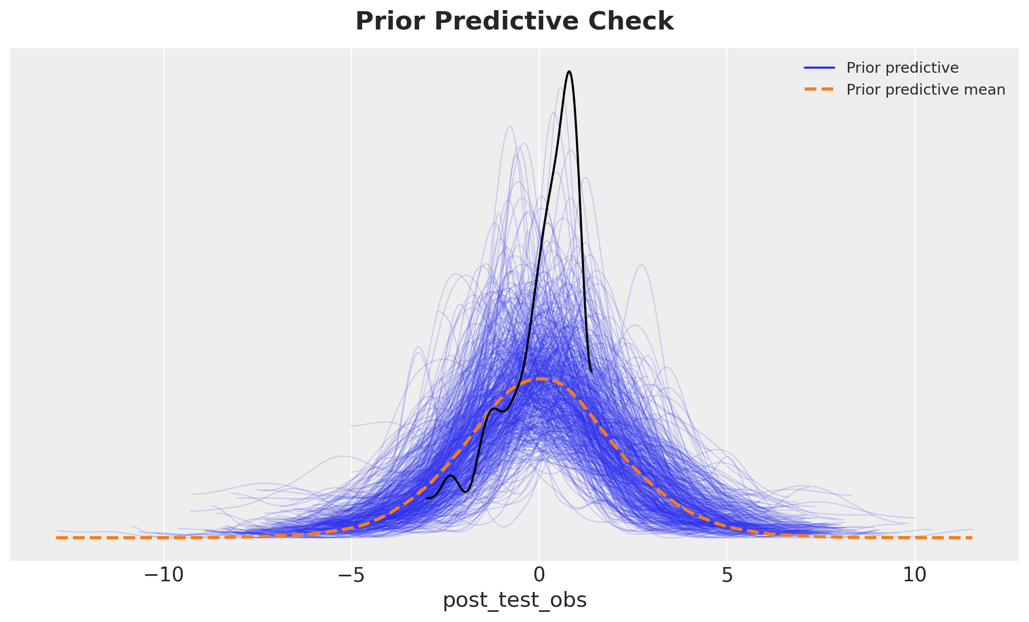
The prior predictive distribution (blue) is compared against the observed data (black). The priors allow for a wide range of plausible outcomes, which is appropriate given our standardized data. The overlap indicates that the observed data are not surprising under our prior assumptions.
Posterior Inference
We now fit the model using Hamiltonian Monte Carlo (HMC) via the NumPyro backend.
with model:
    idata.extend(
        pm.sample(
            tune=1_500,
            draws=1_000,
            target_accept=0.9,
            chains=4,
            nuts_sampler="numpyro",
            random_seed=rng,
        )
    )

    idata.extend(pm.sample_posterior_predictive(idata, random_seed=rng))
After sampling, we generate posterior predictive samples to assess model fit. These predictions will be used to evaluate how well the model captures the observed data patterns.
Model Diagnostics
We check for sampling pathologies that would indicate problems with the posterior geometry or sampler configuration. The primary diagnostic is the number of divergent transitions, which should ideally be zero.
idata["sample_stats"]["diverging"].sum().item()0No divergent transitions indicate that the sampler successfully explored the posterior without encountering problematic curvature. We also examine the summary statistics and trace plots to assess convergence.
az.summary(
    idata,
    var_names=[
        "beta_x",
        "mu_alpha",
        "sigma_alpha",
        "sigma_outcome",
        "theta",
    ],
)| mean | sd | hdi_3% | hdi_97% | mcse_mean | mcse_sd | ess_bulk | ess_tail | r_hat | |
|---|---|---|---|---|---|---|---|---|---|
| beta_x[1, pre_test] | 1.497 | 0.538 | 0.513 | 2.540 | 0.010 | 0.009 | 3137.0 | 2505.0 | 1.0 |
| beta_x[2, pre_test] | 1.547 | 0.113 | 1.342 | 1.766 | 0.002 | 0.002 | 2380.0 | 2645.0 | 1.0 |
| beta_x[3, pre_test] | 1.308 | 0.080 | 1.152 | 1.455 | 0.001 | 0.001 | 3142.0 | 2900.0 | 1.0 |
| beta_x[4, pre_test] | 1.275 | 0.088 | 1.110 | 1.439 | 0.002 | 0.001 | 2369.0 | 2686.0 | 1.0 |
| mu_alpha[1] | 0.887 | 0.897 | -0.699 | 2.686 | 0.016 | 0.015 | 3234.0 | 2615.0 | 1.0 |
| mu_alpha[2] | -0.152 | 0.054 | -0.256 | -0.052 | 0.001 | 0.001 | 2625.0 | 3078.0 | 1.0 |
| mu_alpha[3] | -0.401 | 0.064 | -0.518 | -0.277 | 0.001 | 0.001 | 3139.0 | 2862.0 | 1.0 |
| mu_alpha[4] | -0.460 | 0.088 | -0.621 | -0.297 | 0.002 | 0.001 | 2601.0 | 2761.0 | 1.0 |
| sigma_alpha[1] | 0.639 | 0.140 | 0.382 | 0.908 | 0.004 | 0.003 | 1209.0 | 1328.0 | 1.0 |
| sigma_alpha[2] | 0.219 | 0.054 | 0.122 | 0.329 | 0.002 | 0.002 | 738.0 | 608.0 | 1.0 |
| sigma_alpha[3] | 0.054 | 0.034 | 0.000 | 0.111 | 0.001 | 0.000 | 1082.0 | 1789.0 | 1.0 |
| sigma_alpha[4] | 0.063 | 0.031 | 0.000 | 0.111 | 0.001 | 0.000 | 795.0 | 1340.0 | 1.0 |
| sigma_outcome[1] | 0.460 | 0.084 | 0.317 | 0.617 | 0.002 | 0.002 | 1378.0 | 1483.0 | 1.0 |
| sigma_outcome[2] | 0.230 | 0.032 | 0.171 | 0.288 | 0.001 | 0.001 | 953.0 | 790.0 | 1.0 |
| sigma_outcome[3] | 0.133 | 0.019 | 0.099 | 0.168 | 0.000 | 0.000 | 2446.0 | 2962.0 | 1.0 |
| sigma_outcome[4] | 0.111 | 0.018 | 0.081 | 0.145 | 0.000 | 0.000 | 1293.0 | 2408.0 | 1.0 |
| theta[1] | 0.471 | 0.142 | 0.214 | 0.746 | 0.002 | 0.003 | 7284.0 | 2777.0 | 1.0 |
| theta[2] | 0.235 | 0.058 | 0.127 | 0.345 | 0.001 | 0.001 | 4686.0 | 2972.0 | 1.0 |
| theta[3] | 0.108 | 0.043 | 0.025 | 0.185 | 0.001 | 0.001 | 5843.0 | 2914.0 | 1.0 |
| theta[4] | 0.094 | 0.035 | 0.030 | 0.165 | 0.000 | 0.001 | 6175.0 | 2700.0 | 1.0 |
The summary statistics show effective sample sizes (ESS) and \(\hat{R}\) diagnostics for key parameters. Values of \(\hat{R} \approx 1\) indicate convergence across chains. The treatment effect parameter (theta) and variance components are our main interest.
axes = az.plot_trace(
    idata,
    var_names=[
        "beta_x",
        "mu_alpha",
        "sigma_alpha",
        "sigma_outcome",
        "theta",
    ],
    figsize=(10, 8),
)


plt.gcf().suptitle("Model Trace", fontsize=18, fontweight="bold", y=1.02);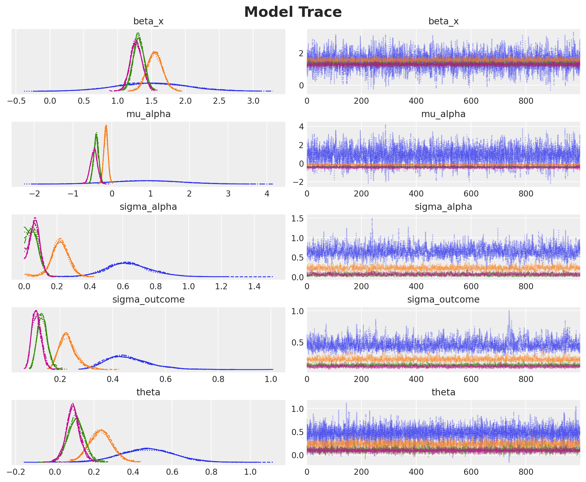
The trace plots show good mixing across chains (overlapping colors) and stable posterior distributions (smooth histograms on the left). The chains have converged to stationary distributions, confirming the reliability of our posterior estimates.
Next, we check the posterior predictive distribution.
fig, ax = plt.subplots()
az.plot_ppc(idata, group="posterior", num_pp_samples=500, ax=ax)
ax.set_title("Posterior Predictive Check", fontsize=18, fontweight="bold", y=1.02);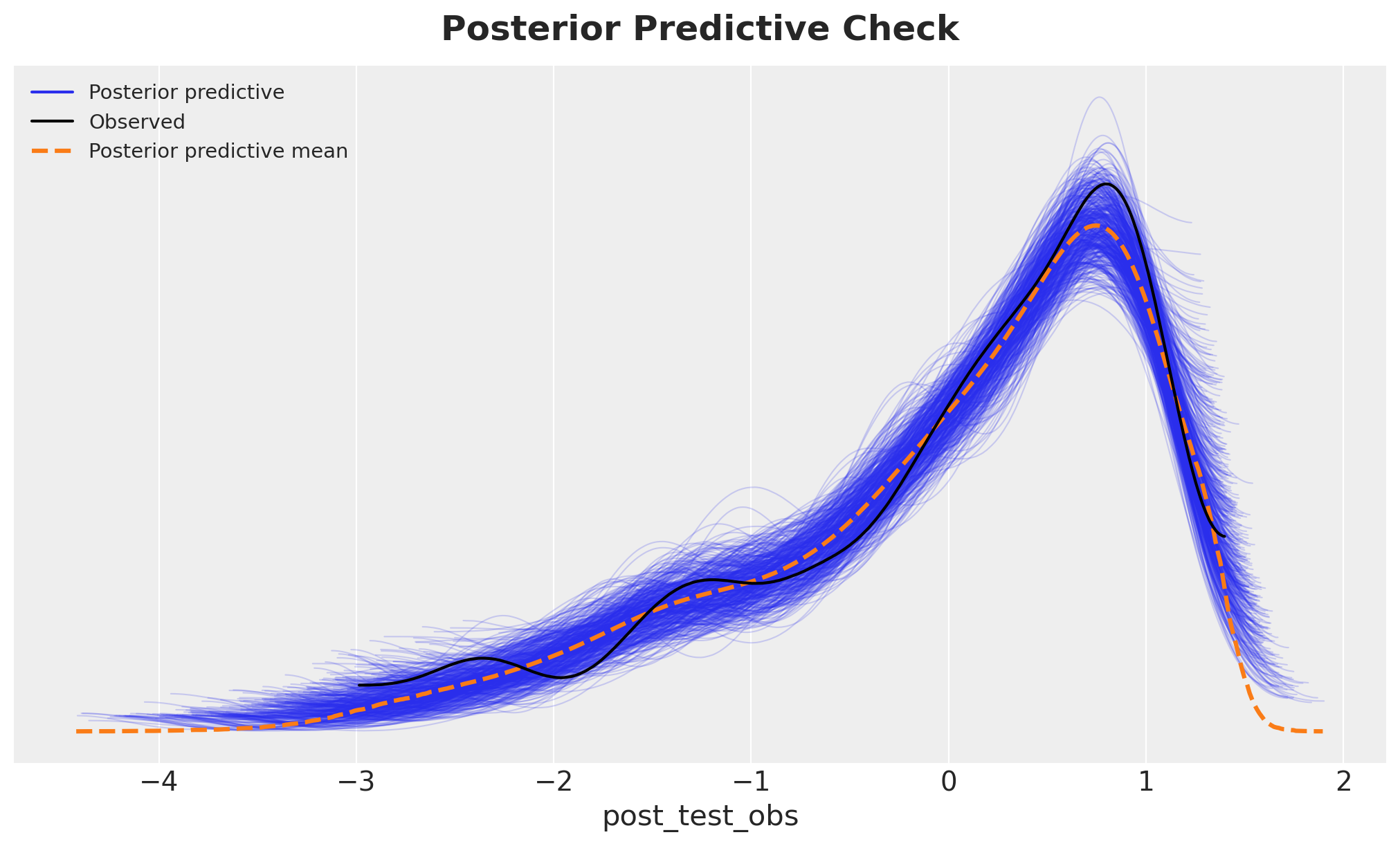
The posterior predictive distribution closely matches the observed data, indicating that the model captures the essential features of the data-generating process.
Treatment Effect Estimates
We now examine the estimated treatment effects. The parameter theta represents the average causal effect of watching “The Electric Company” on standardized test scores, estimated separately for each grade level.
ax, *_ = az.plot_forest(
    idata,
    combined=True,
    var_names=["theta"],
    figsize=(10, 6),
)
ax.set_title(
    r"Treatment Effect Estimates $(94\% HDI)$",
    fontsize=18,
    fontweight="bold",
    y=1.02,
);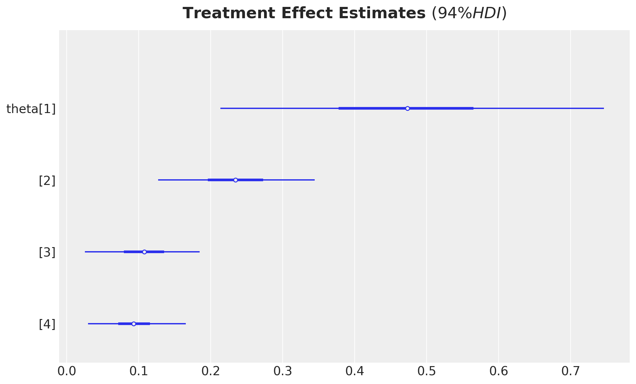
The forest plot shows the posterior distributions of treatment effects for each grade. The point estimates and credible intervals provide evidence about the magnitude and uncertainty of the causal effect. To interpret these effects in the original scale, we transform them back from standardized units.
ax, *_ = az.plot_forest(
    idata["posterior"]["theta"]
    * preprocessor["num"].scale_[numeric_features.index("post_test")],
    combined=True,
    var_names=["theta"],
    figsize=(10, 6),
)
ax.set_title(
    r"Treatment Effect Estimates $(94\% HDI)$ (Original Scale)",
    fontsize=18,
    fontweight="bold",
    y=1.02,
);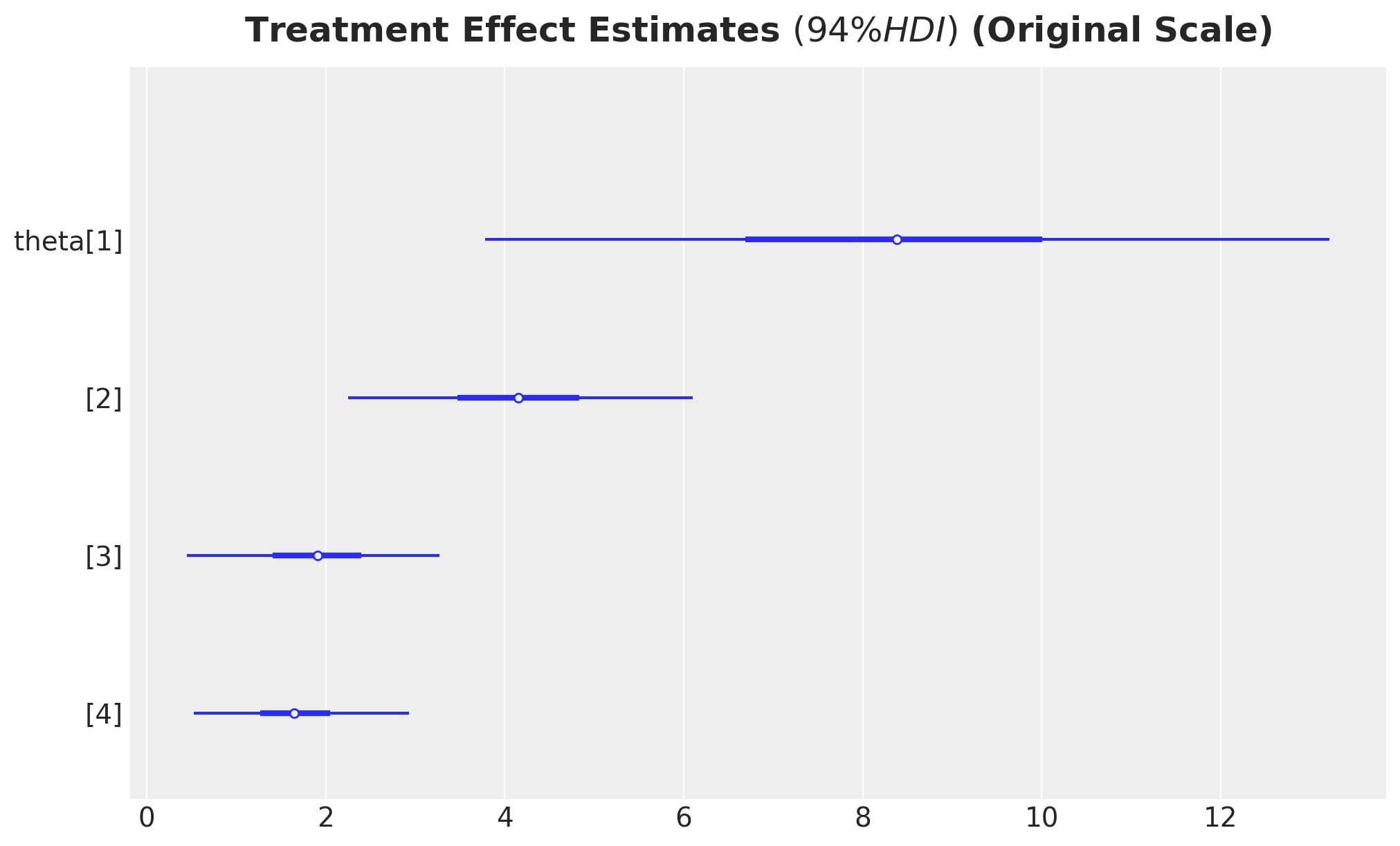
These are the treatment effects expressed in the original units of the test scores. Positive values indicate that the treatment group (who watched the show) scored higher on average than the control group. These values match the results from the book.
Counterfactual Prediction Grids
Here we want to show another way to compute the average treatment effect (ATE) using the marginaleffects package and PyMC do operator to generate counterfactual predictions.
We construct balanced prediction grids that span the range of pre-test scores for both treatment and control conditions. This allows us to compute counterfactual predictions: what would have happened to the same students under both treatment and control.
Remark: We can use the real data instead of the prediction grid. However, this is unnecessary and potentially computationally expensive if the data is large.
# Construct prediction grids (control)
raw_df_control_grid = datagrid(
    newdata=raw_df,
    treatment=0,
    grade=preprocessor["ord"].categories_[ordinal_features.index("grade")],
    pair_id=preprocessor["ord"].categories_[ordinal_features.index("pair_id")],
    pre_test=np.linspace(raw_df["pre_test"].min(), raw_df["pre_test"].max(), 10),
)
# Preprocess the prediction grid
df_control_grid = preprocessor.transform(raw_df_control_grid)
df_control_grid.columns = [col.split("__")[-1] for col in df_control_grid.columns]
x_df_control_grid = df_control_grid[x_columns]

# Construct prediction grids (treatment)
raw_df_treatment_grid = datagrid(
    newdata=raw_df,
    treatment=1,
    grade=preprocessor["ord"].categories_[ordinal_features.index("grade")],
    pair_id=preprocessor["ord"].categories_[ordinal_features.index("pair_id")],
    pre_test=np.linspace(raw_df["pre_test"].min(), raw_df["pre_test"].max(), 10),
)
# Preprocess the prediction grid
df_treatment_grid = preprocessor.transform(raw_df_treatment_grid)
df_treatment_grid.columns = [col.split("__")[-1] for col in df_treatment_grid.columns]
x_df_treatment_grid = df_treatment_grid[x_columns]
We have created two grids: one with treatment set to 0 (control) and one with treatment set to 1 (treated), both spanning the observed range of pre-test scores and all grade-pair combinations.
Counterfactual Estimates
We now generate posterior predictive samples under each counterfactual scenario. For the control grid, we predict outcomes as if all students were in the control condition. For the treatment grid, we predict outcomes as if all students watched the show.
with model:
    pm.set_data(
        new_data={
            "x_data": x_df_control_grid,
            "grade_idx_data": df_control_grid["grade"].to_numpy(),
            "pair_idx_data": df_control_grid["pair_id"].to_numpy(),
            "treatment_data": df_control_grid["treatment"].to_numpy(),
            "post_test_data": df_control_grid["post_test"].to_numpy(),
        },
        coords={
            "covariates": x_df_control_grid.columns,
            "grade": preprocessor["ord"].categories_[ordinal_features.index("grade")],
            "pair_id": preprocessor["ord"].categories_[
                ordinal_features.index("pair_id")
            ],
            "obs_idx": np.arange(len(df_control_grid)),
        },
    )

    posterior_predictive_control = pm.sample_posterior_predictive(
        idata, var_names=["post_test_obs", "mu_outcome"], random_seed=rng
    )
The control counterfactual predictions represent the expected outcomes in the absence of treatment, conditioning on the observed covariates and the estimated model parameters.
with model:
    pm.set_data(
        new_data={
            "x_data": x_df_treatment_grid,
            "grade_idx_data": df_treatment_grid["grade"].to_numpy(),
            "pair_idx_data": df_treatment_grid["pair_id"].to_numpy(),
            "treatment_data": df_treatment_grid["treatment"].to_numpy(),
            "post_test_data": df_treatment_grid["post_test"].to_numpy(),
        },
        coords={
            "covariates": x_df_treatment_grid.columns,
            "grade": preprocessor["ord"].categories_[ordinal_features.index("grade")],
            "pair_id": preprocessor["ord"].categories_[
                ordinal_features.index("pair_id")
            ],
            "obs_idx": np.arange(len(df_treatment_grid)),
        },
    )

    posterior_predictive_treatment = pm.sample_posterior_predictive(
        idata, var_names=["post_test_obs", "mu_outcome"], random_seed=rng
    )
Similarly, the treatment counterfactual predictions represent expected outcomes if all students had watched the show. The difference between these two counterfactuals yields the causal effect.
Results: Treatment Effect Estimates
We can now compute the average treatment effect (ATE) by comparing the posterior predictive distributions under the counterfactual scenarios (Treatment vs. Control). The difference between these predictions, averaged across all observations in the grid, provides a distribution for the causal effect.
For illustration, we focus on Grade 1 students. We first extract and transform the predictions back to the original scale of test scores.
control_mask = (
    raw_df_control_grid.select(pl.col("grade").eq(pl.lit(1))).to_numpy().flatten()
)
control_posterior_grade = posterior_predictive_control["posterior_predictive"][
    "mu_outcome"
][:, :, control_mask]

original_scale_control_posterior_grade = (
    control_posterior_grade
    * preprocessor["num"].scale_[numeric_features.index("post_test")]
    + preprocessor["num"].mean_[numeric_features.index("post_test")]
)

treatment_mask = (
    raw_df_treatment_grid.select(pl.col("grade").eq(pl.lit(1))).to_numpy().flatten()
)
treatment_posterior_grade = posterior_predictive_treatment["posterior_predictive"][
    "mu_outcome"
][:, :, treatment_mask]

original_scale_treatment_posterior_grade = (
    treatment_posterior_grade
    * preprocessor["num"].scale_[numeric_features.index("post_test")]
    + preprocessor["num"].mean_[numeric_features.index("post_test")]
)
We now visualize the posterior distribution of the average treatment effect for Grade 1. The first plot shows the effect computed from the counterfactual predictions, while the second shows the direct coefficient estimate. These should be consistent, providing a validation of our approach.
fig, ax = plt.subplots(
    nrows=2,
    ncols=1,
    sharex=True,
    sharey=True,
    figsize=(10, 8),
    layout="constrained",
)


az.plot_posterior(
    (
        original_scale_treatment_posterior_grade
        - original_scale_control_posterior_grade
    ).mean(dim=("obs_idx")),
    ref_val=0,
    ax=ax[0],
)
ax[0].set(title="ATE from Counterfactual Predictions")

az.plot_posterior(
    (
        idata["posterior"]["theta"]
        * preprocessor["num"].scale_[numeric_features.index("post_test")]
    ).sel(grade=1),
    ref_val=0,
    ax=ax[1],
)
ax[1].set(
    title="ATE from Parameter Estimates (beta coefficient)",
    xlabel="ATE (Original Scale)",
);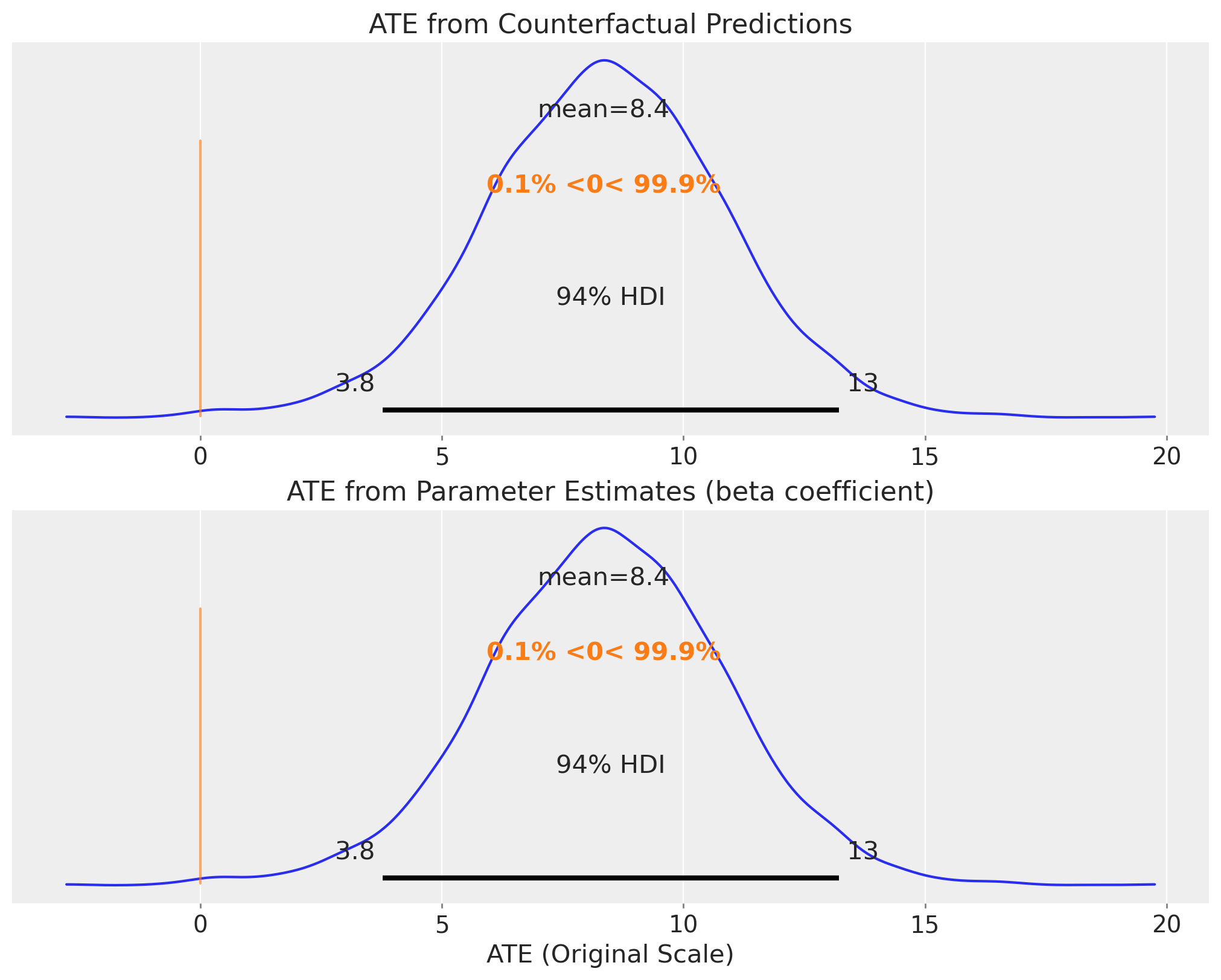
Both approaches yield similar posterior distributions, confirming the robustness of our causal effect estimate. The positive treatment effect indicates that watching “The Electric Company” improved reading scores for Grade 1 students. The credible intervals quantify our uncertainty about the magnitude of this effect.
Part 2: Covariance Model
Motivation: Modeling Treatment Effect Heterogeneity
The hierarchical intercept model in Part 1 assumes that the treatment effect is constant across all pairs (after accounting for grade differences). While this model efficiently controls for pair-level confounding, it does not allow us to explore whether the treatment effect varies across pairs. In practice, some schools or classrooms may respond more strongly to the intervention than others due to unmeasured factors such as teacher implementation fidelity, student engagement, or local context.
To capture this treatment effect heterogeneity, we extend our model to allow both the baseline intercept \(\alpha_j\) and the treatment effect \(\theta_j\) to vary across pairs. Moreover, we model the joint distribution of these pair-specific parameters using a bivariate normal distribution with a covariance structure:
\[ \begin{pmatrix} \alpha_j \\ \theta_j \end{pmatrix} \sim \text{MvNormal}\left(\begin{pmatrix} \mu_\alpha \\ \mu_\theta \end{pmatrix}, \Sigma\right) \]
where \(\Sigma\) is a \(2 \times 2\) covariance matrix. The off-diagonal elements of \(\Sigma\) capture the correlation between baseline performance and treatment response. For example, a positive correlation would indicate that pairs with higher baseline scores also tend to experience larger treatment effects, while a negative correlation would suggest compensatory effects (treatment helps struggling pairs more).
Benefits of Modeling Covariances
This approach represents what Huntington-Klein (2021, The Effect, Chapter 16) calls “Advanced Random Effects” or multi-level modeling. By explicitly modeling the covariance structure, we gain several advantages over both standard Fixed Effects and basic Random Effects:
- Captures heterogeneity: We estimate not just the average treatment effect \(\mu_\theta\), but also the distribution of pair-specific effects \(\theta_j\), revealing how treatment impacts vary across contexts.
- Partial pooling on treatment effects: Noisy pair-specific estimates are shrunk toward the population mean, borrowing strength across groups. This provides more stable estimates than treating each pair entirely separately.
- Correlation structure: We learn whether baseline performance and treatment response are related, which can inform targeting and generalization of the intervention. This addresses the limitation of basic Random Effects by explicitly modeling the relationship between group characteristics and effects.
- Separation of between and within effects: By allowing both intercepts and slopes to vary, we can distinguish population-level patterns from group-specific deviations, providing richer substantive interpretation.
- Efficiency with hierarchical data: Multi-level models make full use of the hierarchical structure, improving statistical efficiency compared to Fixed Effects while relaxing the strong independence assumptions of basic Random Effects.
We implement this model using a non-centered parametrization with a Cholesky decomposition of the covariance matrix for computational efficiency. We follow closely the approach described in the (great!) blog post Hierarchical modeling with the LKJ prior in PyMC by Tomi Capretto.
There is a small caveat though: PyMC does not allow us (yet) to vectorize the LKJ prior. So we need to do it manually. Which in this case is relatively easy as we just have one correlation factor to vectorize (so we simply use a shifted Beta distribution).
The following helper functions construct correlation and covariance matrices in a vectorized manner for each grade level.
def vectorized_correlation_matrices(corr_values, size=2):
    n_matrices = corr_values.shape[0]

    # Reshape for broadcasting
    # Use reshape or expand_dims instead of dimshuffle
    corr_expanded = pt.reshape(corr_values, (n_matrices, 1, 1))

    # Create base: all elements are correlation values
    base = corr_expanded * pt.ones((n_matrices, size, size))

    # Create diagonal mask
    diag_mask = pt.eye(size, dtype="bool")

    # Set diagonal to 1
    return pt.where(diag_mask, 1.0, base)


def vectorized_diagonal_matrices_v4(values):
    k = values.shape[1]  # 2

    # Create identity matrix (2, 2)
    identity_matrix = pt.eye(k)

    # Reshape values for broadcasting: (4, 2) -> (4, 2, 1)
    values_expanded = values[:, :, None]

    # Multiply: (4, 2, 1) * (2, 2) -> (4, 2, 2)
    # This puts values[i, j] at position [i, j, j]
    return values_expanded * identity_matrix
Prior Specification for Correlation
Before specifying the full model, we visualize our prior distribution for the correlation parameter. We use a \(\text{Beta}(20, 5)\) distribution (scaled to \([-1, 1]\)) to encode a prior belief that the correlation between intercepts and treatment effects is likely positive but with substantial uncertainty. This prior is weakly informative and allows the data to dominate the posterior inference.
pz.Beta(alpha=20, beta=5).plot_pdf(pointinterval=True);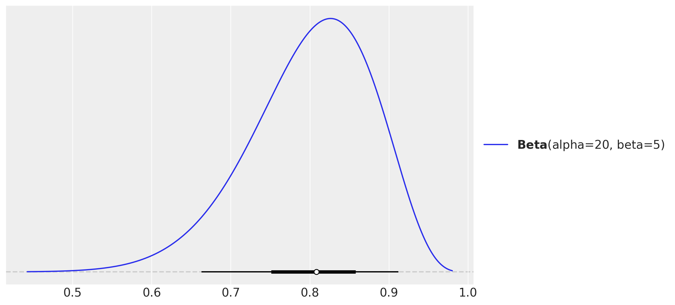
The Beta distribution shown above is transformed to the correlation scale via the mapping \(\psi = 2 \times \text{Beta}(20, 5) - 1\). This induces a prior that favors positive correlations but remains flexible enough to accommodate a range of values.
Model Specification
We now specify the full covariance model. The key difference from Part 1 is that both the intercept and the treatment effect vary by pair. The model structure is:
\[ \begin{align} \text{post_test}_i &\sim \text{Normal}(\mu_i, \sigma_y) \\ \mu_i &= \alpha_{\text{pair}[i]} + \theta_{\text{pair}[i]} \cdot T_i + \beta_x \cdot \text{pre_test}_i \\ \begin{pmatrix} \alpha_j \\ \theta_j \end{pmatrix} &\sim \text{Normal}\left(\begin{pmatrix} \mu_\alpha \\ \mu_\theta \end{pmatrix}, \Sigma\right) \end{align} \]
where \(\Sigma\) is decomposed as \(\Sigma = D \Omega D\), with \(D\) being a diagonal matrix of standard deviations and \(\Omega\) being the correlation matrix. This decomposition allows us to place separate priors on the marginal variances and the correlation structure, which improves interpretability and sampling efficiency.
As in the model in Part 1, we use a non-centered parametrization to improve sampling efficiency.
coords.update({"effect": ["intercept", "slope"], "effect_copy": ["intercept", "slope"]})
coords.update({"corr_dim": ["corr_dim_1"]})

with pm.Model(coords=coords) as cov_model:
    # --- Data Containers ---
    # covariates
    x_data = pm.Data("x_data", x_df, dims=("obs_idx", "covariates"))
    # grade
    grade_idx_data = pm.Data("grade_idx_data", df["grade"].to_numpy(), dims="obs_idx")
    # object categories
    pair_idx_data = pm.Data("pair_idx_data", df["pair_id"].to_numpy(), dims="obs_idx")
    # treatment
    treatment_data = pm.Data(
        "treatment_data", df["treatment"].to_numpy(), dims=("obs_idx")
    )
    # outcome
    post_test_data = pm.Data(
        "post_test_data", df["post_test"].to_numpy(), dims="obs_idx"
    )

    # --- Priors ---

    beta_x = pm.Normal("beta_x", mu=0, sigma=1, dims=("grade", "covariates"))
    sigma_outcome = pm.HalfNormal("sigma_outcome", sigma=1, dims=("grade"))

    mu_alpha = pm.Normal("mu_alpha", mu=0, sigma=0.5, dims=("grade"))
    mu_theta = pm.Normal("mu_theta", mu=0, sigma=0.5, dims=("grade"))

    # Group-level standard deviations
    sigma_u = pm.HalfNormal(
        "sigma_u", sigma=np.array([0.2, 0.2]), dims=("grade", "effect")
    )

    # Triangular upper part of the correlation matrix
    # omega_triu = pm.LKJCorr("omega_triu", eta=1, n=2, dims=("grade", "corr_dim")) <- Not supported yet! # noqa: E501
    omega_triu = pm.Beta("omega_triu", alpha=20, beta=5, dims=("grade", "corr_dim"))
    omega_triu_scaled = pm.Deterministic(
        "omega_triu_scaled", omega_triu * 2 - 1, dims=("grade", "corr_dim")
    )

    # Construct correlation matrix
    omega = pm.Deterministic(
        "omega",
        vectorized_correlation_matrices(omega_triu_scaled),
        dims=("grade", "effect", "effect_copy"),
    )

    # Construct diagonal matrix of standard deviation
    sigma_diagonal = pm.Deterministic(
        "sigma_diagonal",
        vectorized_diagonal_matrices_v4(sigma_u),
        dims=("grade", "effect", "effect_copy"),
    )

    # Compute covariance matrix
    cov = pm.Deterministic(
        "cov",
        pt.einsum("bij,bjk,bkl->bil", sigma_diagonal, omega, sigma_diagonal),
        dims=("grade", "effect", "effect_copy"),
    )

    # Cholesky decomposition of covariance matrix
    cholesky_cov = pm.Deterministic(
        "cholesky_cov",
        pt.slinalg.cholesky(cov),
        dims=("grade", "effect", "effect_copy"),
    )

    # And finally get group-specific coefficients
    u_raw = pm.Normal("u_raw", mu=0, sigma=1, dims=("grade", "effect", "pair_id"))
    u = pm.Deterministic(
        "u",
        pt.einsum("bik,bkj->bji", cholesky_cov, u_raw),
        dims=("grade", "pair_id", "effect"),
    )

    # Extract the intercept and slope components deviations from the population means
    u0 = pm.Deterministic("u0", u[:, :, 0], dims=("grade", "pair_id"))
    u1 = pm.Deterministic("u1", u[:, :, 1], dims=("grade", "pair_id"))

    # Extract the intercept and slope components
    alpha = pm.Deterministic("alpha", mu_alpha + u0.T, dims=("pair_id", "grade"))
    theta = pm.Deterministic("theta", mu_theta + u1.T, dims=("pair_id", "grade"))

    mu_outcome = pm.Deterministic(
        "mu_outcome",
        alpha[pair_idx_data, grade_idx_data]
        + theta[pair_idx_data, grade_idx_data] * treatment_data
        + (beta_x[grade_idx_data] * x_data).sum(axis=-1),
        dims=("obs_idx"),
    )

    # --- Likelihood ---
    pm.Normal(
        "post_test_obs",
        mu=mu_outcome,
        sigma=sigma_outcome[grade_idx_data],
        observed=post_test_data,
        dims="obs_idx",
    )

pm.model_to_graphviz(cov_model)
Prior Predictive Check
As in Part 1, we sample from the prior distribution to verify that our priors produce reasonable predictions before observing the data. This is especially important for the covariance model, where the additional flexibility could lead to implausible outcomes if priors are poorly calibrated.
with cov_model:
    cov_idata = pm.sample_prior_predictive(random_seed=rng)

fig, ax = plt.subplots()
az.plot_ppc(cov_idata, group="prior", ax=ax)
az.plot_dist(df["post_test"].to_numpy(), color="black", ax=ax)
ax.set_title(
    "Prior Predictive Check - Covariance Model", fontsize=18, fontweight="bold", y=1.02
);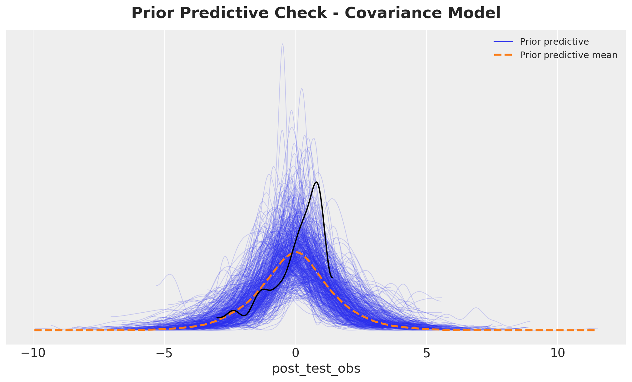
This prior predictive distribution looks quite reasonable.
Posterior Inference
We now fit the covariance model using HMC. Due to the increased complexity of the model (additional parameters and correlation structure), we use a longer tuning phase (2,000 iterations) and a higher target acceptance rate (0.95) to ensure thorough exploration of the posterior geometry.
with cov_model:
    cov_idata.extend(
        pm.sample(
            tune=2_000,
            draws=1_000,
            chains=4,
            nuts_sampler="numpyro",
            target_accept=0.95,
            random_seed=rng,
        )
    )

    cov_idata.extend(pm.sample_posterior_predictive(cov_idata))
Posterior sampling is complete without any issues.
Model Diagnostics
We examine diagnostic statistics to ensure the sampler converged successfully. The covariance model has a more complex posterior geometry, so careful attention to diagnostics is essential.
cov_idata["sample_stats"]["diverging"].sum().item()0The absence of divergent transitions indicates successful sampling. The more complex model structure did not cause problematic posterior geometry, which validates our use of the non-centered parametrization and appropriate tuning parameters.
Next, let’s check the posterior predictive distribution.
fig, ax = plt.subplots()
az.plot_ppc(cov_idata, group="posterior", num_pp_samples=500, ax=ax)
ax.set_title(
    "Posterior Predictive Check - Covariance Model",
    fontsize=18,
    fontweight="bold",
    y=1.02,
);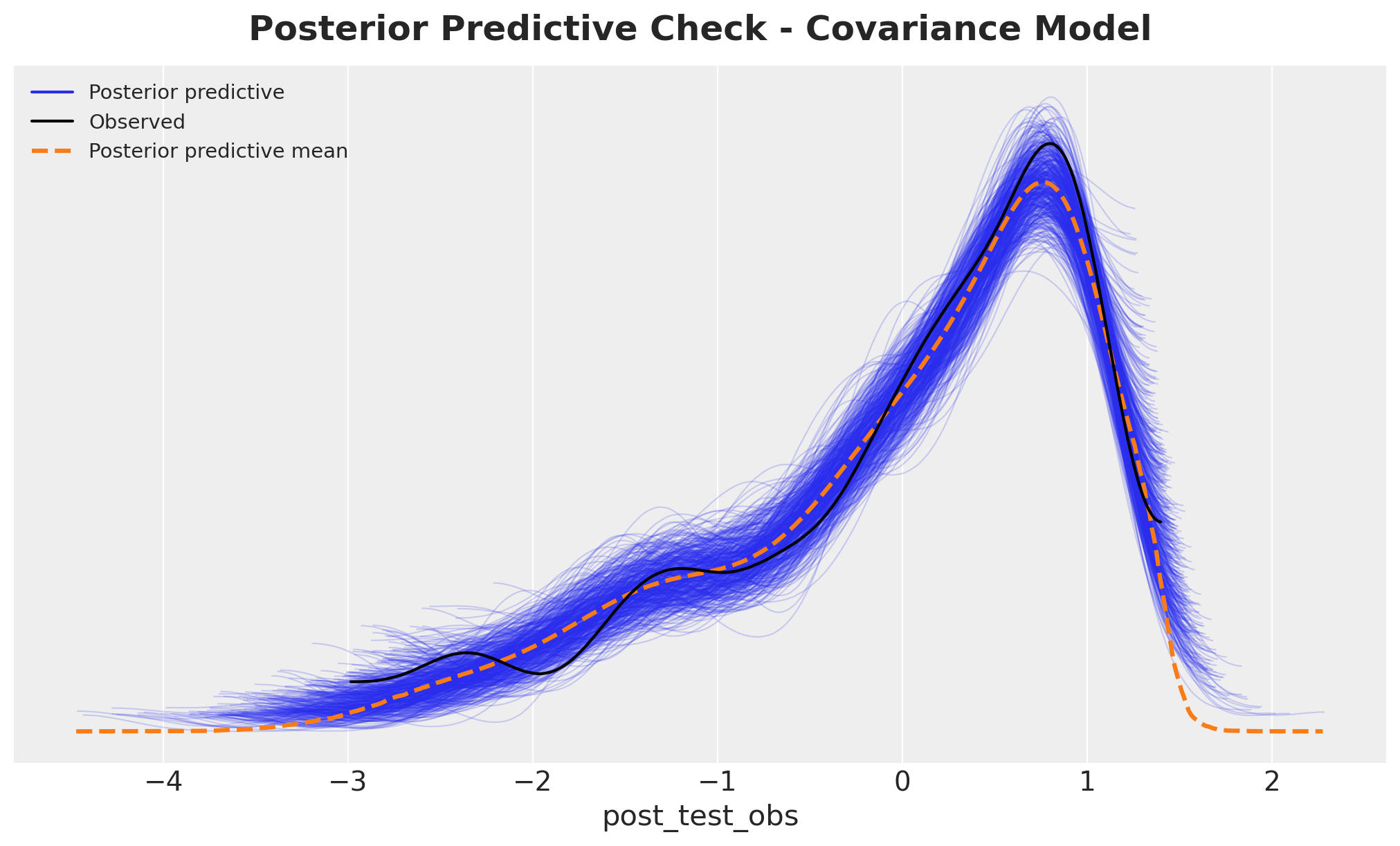
Overall, the posterior predictive distribution looks good.
As the key ingredient of the covariance model is the correlation parameter, let’s visualize the posterior distribution of the correlation parameter and compare it to the prior.
axes = az.plot_dist_comparison(
    cov_idata,
    var_names=["omega_triu_scaled"],
    figsize=(10, 18),
)
plt.gcf().suptitle(
    "Prior vs Posterior Comparison - Covariance Model",
    fontsize=18,
    fontweight="bold",
    y=1.02,
);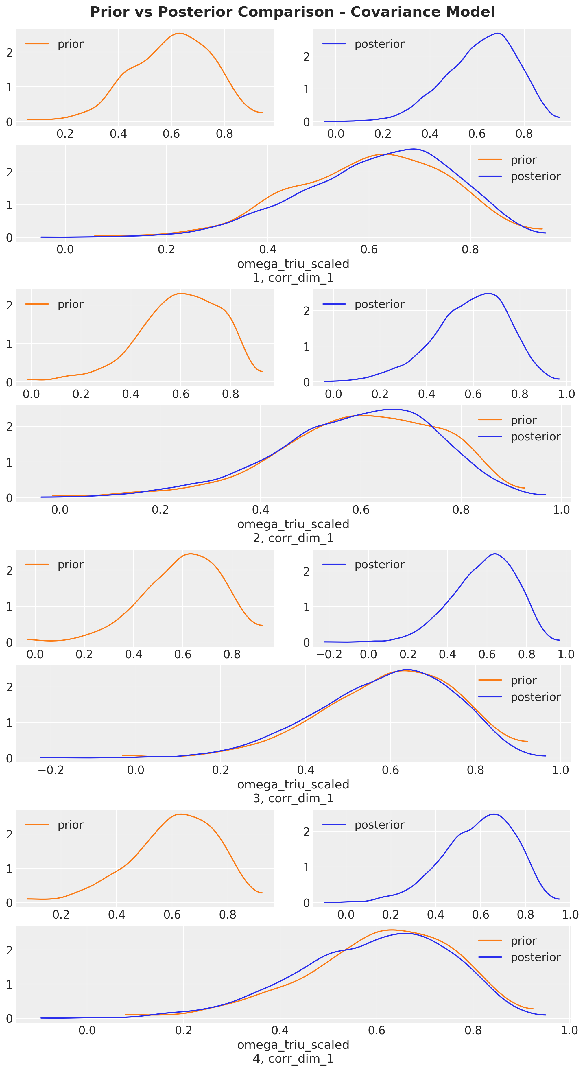
We do not see much difference between the prior and posterior distribution of the correlation parameter. Hence, this shows the covariance structure is not overly influential in the average treatment effect for this example. This is consistent with Gelman and Hill’s findings in their book.
Treatment Effect Estimates
We now examine the estimated treatment effects from the covariance model. Unlike Part 1, where we had a single treatment effect parameter per grade, here we have a population-level mean treatment effect (mu_theta) and pair-specific deviations from this mean (theta). The parameter mu_theta represents the average causal effect across all pairs within a grade.
fig, ax = plt.subplots(
    nrows=2,
    ncols=1,
    sharex=True,
    sharey=True,
    figsize=(10, 8),
    layout="constrained",
)

az.plot_forest(
    idata["posterior"]["theta"]
    * preprocessor["num"].scale_[numeric_features.index("post_test")],
    combined=True,
    var_names=["theta"],
    ax=ax[0],
)
ax[0].set(title="Hierarchical Intercept Model")

az.plot_forest(
    cov_idata["posterior"]["mu_theta"]
    * preprocessor["num"].scale_[numeric_features.index("post_test")],
    combined=True,
    var_names=["mu_theta"],
    ax=ax[1],
)
ax[1].set(title="Covariance Model")
fig.suptitle(
    r"Treatment Effect Estimates $(94\% HDI)$ (Original Scale)",
    fontsize=18,
    fontweight="bold",
    y=1.05,
);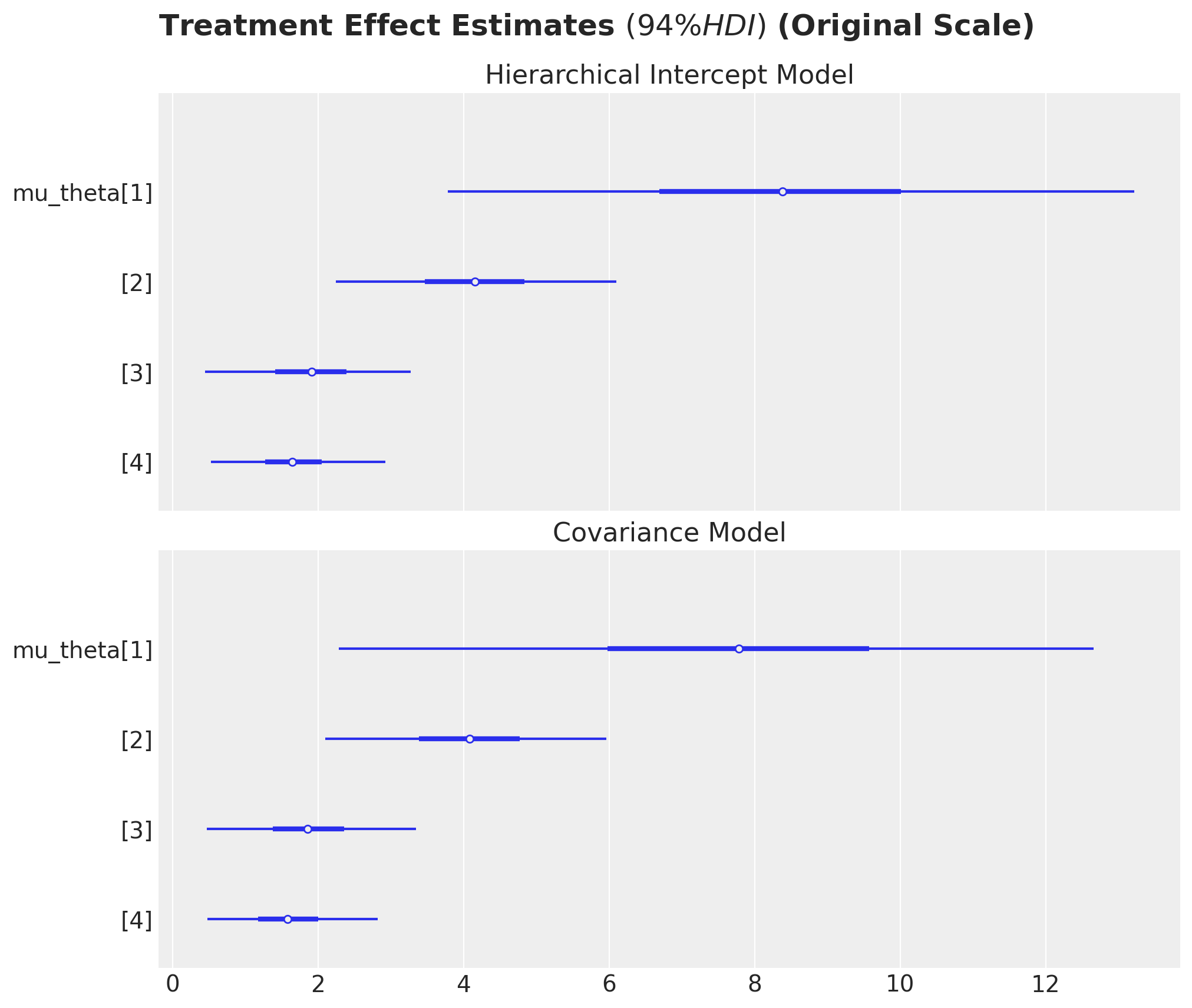
The forest plot shows the posterior distribution of the average treatment effect (mu_theta) for each grade. These estimates are comparable to the theta estimates from Part 1, but they now represent the mean of a distribution of pair-specific effects rather than a fixed common effect.
Hierarchical Shrinkage: Population vs. Group-Level Effects
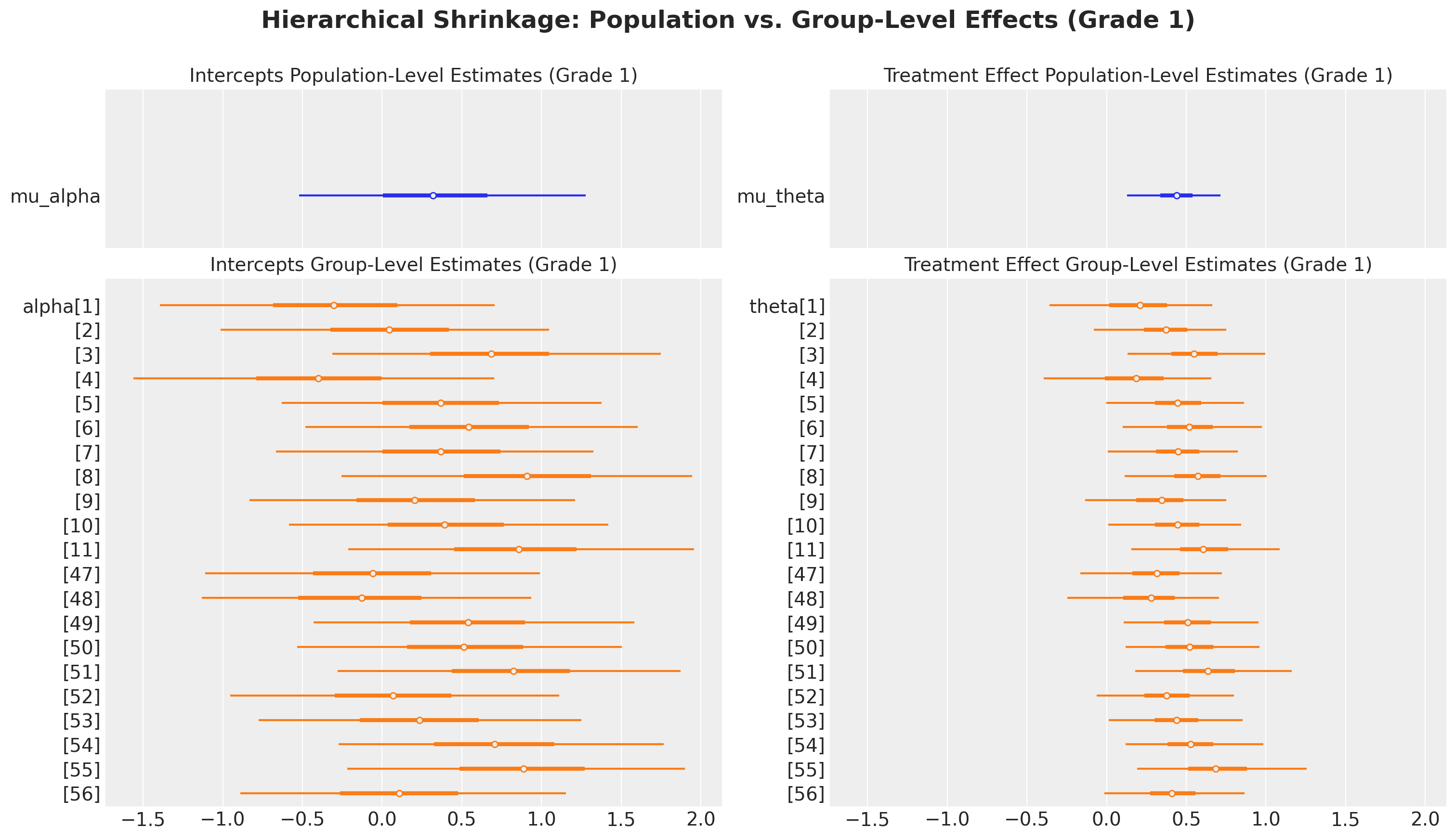
One of the key advantages of the covariance model is that it allows us to estimate both population-level parameters (the means \(\mu_\alpha\) and \(\mu_\theta\)) and group-level parameters (the pair-specific \(\alpha_j\) and \(\theta_j\)). Through partial pooling, the model borrows strength across pairs: estimates for pairs with sparse data are shrunk toward the population mean, while estimates for data-rich pairs are allowed to deviate more.
The visualization below compares population-level and group-level estimates for Grade 1. The top row shows the population means (\(\mu_\alpha\) and \(\mu_\theta\)), while the bottom row shows the distribution of pair-specific effects (\(\alpha_j\) and \(\theta_j\)) for pairs within Grade 1. The degree of shrinkage depends on the estimated between-pair variance: if pairs are highly similar, estimates will be heavily pooled; if pairs differ substantially, estimates will retain more individual variation.
fig, ax = plt.subplots(
    nrows=2,
    ncols=2,
    height_ratios=[0.3, 1],
    figsize=(15, 8),
    sharex=True,
    sharey=False,
    layout="constrained",
)

az.plot_forest(
    cov_idata["posterior"].sel(grade=1),
    combined=True,
    var_names=["mu_alpha"],
    colors="C0",
    ax=ax[0, 0],
)
ax[0, 0].set_title("Intercepts Population-Level Estimates (Grade 1)", fontsize=14)


az.plot_forest(
    cov_idata["posterior"]
    .sel(grade=1)
    .where(
        cov_idata["posterior"].pair_id.isin(
            raw_df.group_by("grade")
            .agg(pl.col("pair_id").unique())
            .filter(pl.col("grade").eq(pl.lit(1)))["pair_id"]
            .to_list()
        ),
        drop=True,
    ),
    var_names=["alpha"],
    combined=True,
    colors="C1",
    ax=ax[1, 0],
)
ax[1, 0].set_title("Intercepts Group-Level Estimates (Grade 1)", fontsize=14)


az.plot_forest(
    cov_idata["posterior"].sel(grade=1),
    combined=True,
    var_names=["mu_theta"],
    colors="C0",
    ax=ax[0, 1],
)
ax[0, 1].set_title("Treatment Effect Population-Level Estimates (Grade 1)", fontsize=14)

az.plot_forest(
    cov_idata["posterior"]
    .sel(grade=1)
    .where(
        cov_idata["posterior"].pair_id.isin(
            raw_df.group_by("grade")
            .agg(pl.col("pair_id").unique())
            .filter(pl.col("grade").eq(pl.lit(1)))["pair_id"]
            .to_list()
        ),
        drop=True,
    ),
    var_names=["theta"],
    combined=True,
    colors="C1",
    ax=ax[1, 1],
)
ax[1, 1].set_title("Treatment Effect Group-Level Estimates (Grade 1)", fontsize=14)
fig.suptitle(
    "Hierarchical Shrinkage: Population vs. Group-Level Effects (Grade 1)",
    fontsize=18,
    fontweight="bold",
    y=1.07,
);
Conclusion
This analysis demonstrates how multilevel models provide a principled framework for causal inference in clustered data, combining the virtues of experimental design with efficient statistical estimation. We estimated the causal effect of watching “The Electric Company” on reading scores using two complementary hierarchical models, each offering distinct insights and tradeoffs.
References
- Gelman, A., & Hill, J. (2006). Data Analysis Using Regression and Multilevel/Hierarchical Models. Cambridge University Press. Chapter 23: Causal Inference Using Multilevel Models.
- Huntington-Klein, N. (2021). The Effect: An Introduction to Research Design and Causality. Chapman and Hall/CRC. Chapter 16: Fixed Effects. Available online at https://theeffectbook.net/ch-FixedEffects.html