Probability that a given observation is part of a bootstrap sample?

Solution of Excercise 5.4.2

Suppose that we obtain a bootstrap sample from a set of \(n\) observations \(x_1, …, x_n\).

(a) What is the probability that the first bootstrap observation is not the \(j\)-th observation from the original sample?

Let us denote this probability by \(_j\). As the probability of selecting a particular \(x_j\) from the set \(x_1, …, x_n\) is \(1/n\), then the desired probability is

\[\begin{equation*} \pi_j = 1-\frac{1}{n} \end{equation*}\]

(b) What is the probability that the second bootstrap observation is not the \(j\)-th observation from the original sample?

Well, it is not hard to see that, as the selections are independent then, this probability is again \(_j\).

(c) Argue that the probability \(p_j(n)\) that the \(j\)-th observation is not in the bootstrap sample is \((1 − 1/n)^n\).

It is straight forward to see from (a) and (b) that this probability is given by

\[\begin{equation*} p_j(n)= \prod_{i=1}^n \pi_j = \left(1-\frac{1}{n}\right)\left(1-\frac{1}{n}\right)\cdots\left(1-\frac{1}{n}\right) =\left(1-\frac{1}{n}\right)^n. \end{equation*}\]

Let us define a function which computes this probability.

def probability(n):
    return (1 - 1/n)**n

(d) When \(n = 5\), what is the probability that the \(j\)-th observation is in the bootstrap sample?

# This is simply:
1 - probability(5)

0.6723199999999999

(e) When \(n = 100\), what is the probability that the \(j\)-th observation is in the bootstrap sample?

1 - probability(100)

0.6339676587267709

(f) When \(n = 10000\), what is the probability that the \(j\)-th observation is in the bootstrap sample?

1 - probability(1e4)

0.6321389535670295

(d) Create a plot that displays, for each integer value of \(n\) from \(1\) to \(100,000\), the probability that the \(j\)-th observation is in the bootstrap sample. Comment on what you observe.

We first do it for \(n\) from \(1\) to \(50\):

import numpy as np
import matplotlib.pyplot as plt
plt.style.use('seaborn')

%matplotlib inline

def generate_plot(sample_size_max):
    
    sample_sizes = np.arange(sample_size_max, dtype=float)

    probability_sequence = [1 - probability(n+1) for n in sample_sizes]
    
    plt.figure(figsize=(9, 7))
    plt.plot(sample_sizes, probability_sequence, marker='o')
    plt.plot(sample_sizes, probability_sequence, color='red')
    plt.title('Probability Sequence')
    plt.xlabel('Sample Size')
    plt.ylabel('probability the j-th observation is in the bootstrap');

generate_plot(50);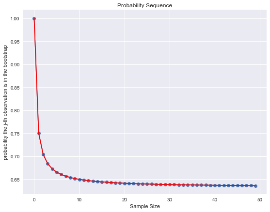

Now we do it for \(n\) from 1 to 100,000:

generate_plot(1e5);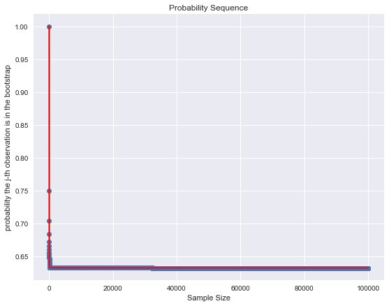

Clearly this probabilities are converging! But, to which value?

Recall that the exponential function satisfies:

\[\begin{equation*} e^x = \lim_{n\rightarrow \infty} \left(1+\frac{x}{n}\right)^n \end{equation*}\]

Hence, we easily see that

\[\begin{equation*} p_j := \lim_{n\rightarrow \infty}p_j(n) = e^{-1} \approx 0.3678794 \end{equation*}\]

Therefore the limit as \(n\) increases of the probability the \(j\)-th observation is in the bootstrap is:

1 - np.exp(-1) # Which is roughly 2/3.

0.6321205588285577

Let us plot this:

generate_plot(50)
plt.axhline(y=1 - np.exp(-1) , color='g', linestyle='--');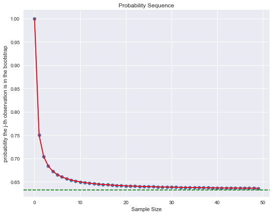

generate_plot(1e5)
plt.axhline(y=1 - np.exp(-1) , color='g', linestyle='--');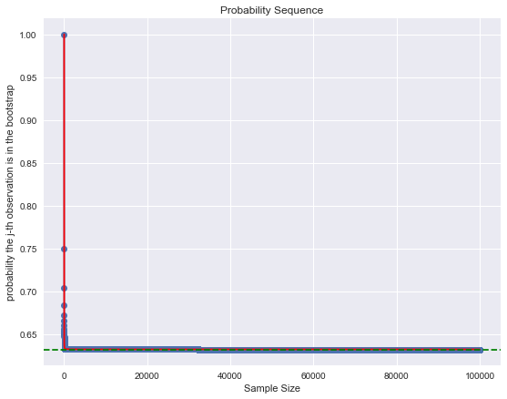

(h) We will now investigate numerically the probability that a bootstrap sample of size \(n = 100\) contains the \(j\)-th observation. Here \(j = 4\). We repeatedly create bootstrap samples, and each time we record whether or not the fourth observation is contained in the bootstrap sample.

We write this function as:

def get_probability(num_iterations, n, j):
    
    sample = [
        (np.random.choice(n, n) == j).sum() > 0 
        for i in range(0, num_iterations)
    ]
    
    sample = np.array(sample)
    
    return sample.mean()

num_iterations = int(1e5)
n = 100
j = 4

sample_mean = get_probability(num_iterations, n, j)
sample_mean

0.63511

This value is quite close to \(1-e^{-1}\).

abs(sample_mean - (1 - np.exp(-1)))

0.0029894411714422864

Let us go a step further as do this computation many times!

def simulation(n, j, N):
    
    simulation_array = [
        get_probability(num_iterations, n, j) 
        for i in range(0, N)
    ]
    
    return np.array(simulation_array)

We run the simulations:

simulation_array = simulation(n, j, N=500)

Let us see the histogram of the samples:

plt.figure(figsize=(9, 7))
plt.hist(simulation_array, bins=30)  
plt.axvline(simulation_array.mean(), color='red', linestyle='--', label='simulation mean')
plt.axvline(1 - np.exp(-1), color='purple', linestyle='--', label='1 - exp(-1)')
plt.legend()
plt.title(f'Histogram:  Bootstrap sample of size n=100 contains the {j}-th observation');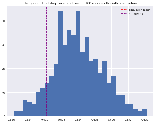

If we compute the mean:

simulation_array.mean()

0.63398918

and compare it with

1 - probability(n)

0.6339676587267709

abs(simulation_array.mean() - (1 - probability(n)))

2.1521273229185844e-05

We get the expected result!