# Univariate forecasting with `numpyro_forecast`
Here we present an introduction to the `numpyro_forecast` package. This notebook ports the blog post [**Univariate time series forecasting with NumPyro**](https://juanitorduz.github.io/numpyro_forecasting-univariate/) (itself a port of Pyro's [forecasting tutorial](https://pyro.ai/examples/forecasting_i.html)) to the [`numpyro_forecast`](https://github.com/juanitorduz/numpyro_forecast) package. We forecast **weekly BART ridership** with a random-walk local level, Fourier seasonality and a Student-T likelihood, fit with stochastic variational inference (SVI), and evaluate with the continuous ranked probability score (CRPS).
Instead of hand-writing the NumPyro model and a bespoke prediction loop, we subclass [numpyro_forecast.forecaster.ForecastingModel](../../../reference/forecaster.ForecastingModel.md#numpyro_forecast.forecaster.ForecastingModel) and let [Forecaster](../../../reference/forecaster.Forecaster.md#numpyro_forecast.forecaster.Forecaster) handle the *fit-once / forecast-any-horizon* mechanics (the forecast horizon is drawn from separate `_future` latent sites, so the variational guide is never resized).
> **Note on reproducibility.** We match the blog's data, seed, optimizer and step counts. Results reproduce the blog's behavior and CRPS magnitude but are not bit-for-bit identical: the forecast horizon uses the package's separate-`_future`-site mechanism (rather than re-running the guide over the full covariates), and the seasonal design uses [fourier_features](../../../reference/features.fourier_features.md#numpyro_forecast.features.fourier_features), an equivalent Fourier basis.
# Prepare notebook
In [1]:
``` python
from functools import partial
from time import perf_counter
import arviz as az
import jax.numpy as jnp
import matplotlib.pyplot as plt
import numpy as np
import numpyro
import numpyro.distributions as dist
from jax import random
from numpyro.infer import Predictive
from numpyro.infer.reparam import LocScaleReparam
from numpyro.optim import Adam
from numpyro_forecast import (
Forecaster,
ForecastingModel,
backtest,
backtest_vectorized,
eval_coverage,
eval_crps,
)
from numpyro_forecast.datasets import load_bart_weekly
from numpyro_forecast.features import fourier_features
from numpyro_forecast.functional import Horizon, forecasting_model, predict, time_series
from numpyro_forecast.typing import Array
az.style.use("arviz-darkgrid")
plt.rcParams["figure.figsize"] = [10, 6]
plt.rcParams["figure.dpi"] = 100
plt.rcParams["figure.facecolor"] = "white"
numpyro.set_host_device_count(n=4)
rng_key = random.PRNGKey(seed=42)
%load_ext autoreload
%autoreload 2
%load_ext jaxtyping
%jaxtyping.typechecker beartype.beartype
%config InlineBackend.figure_format = "retina"
```
# Read data
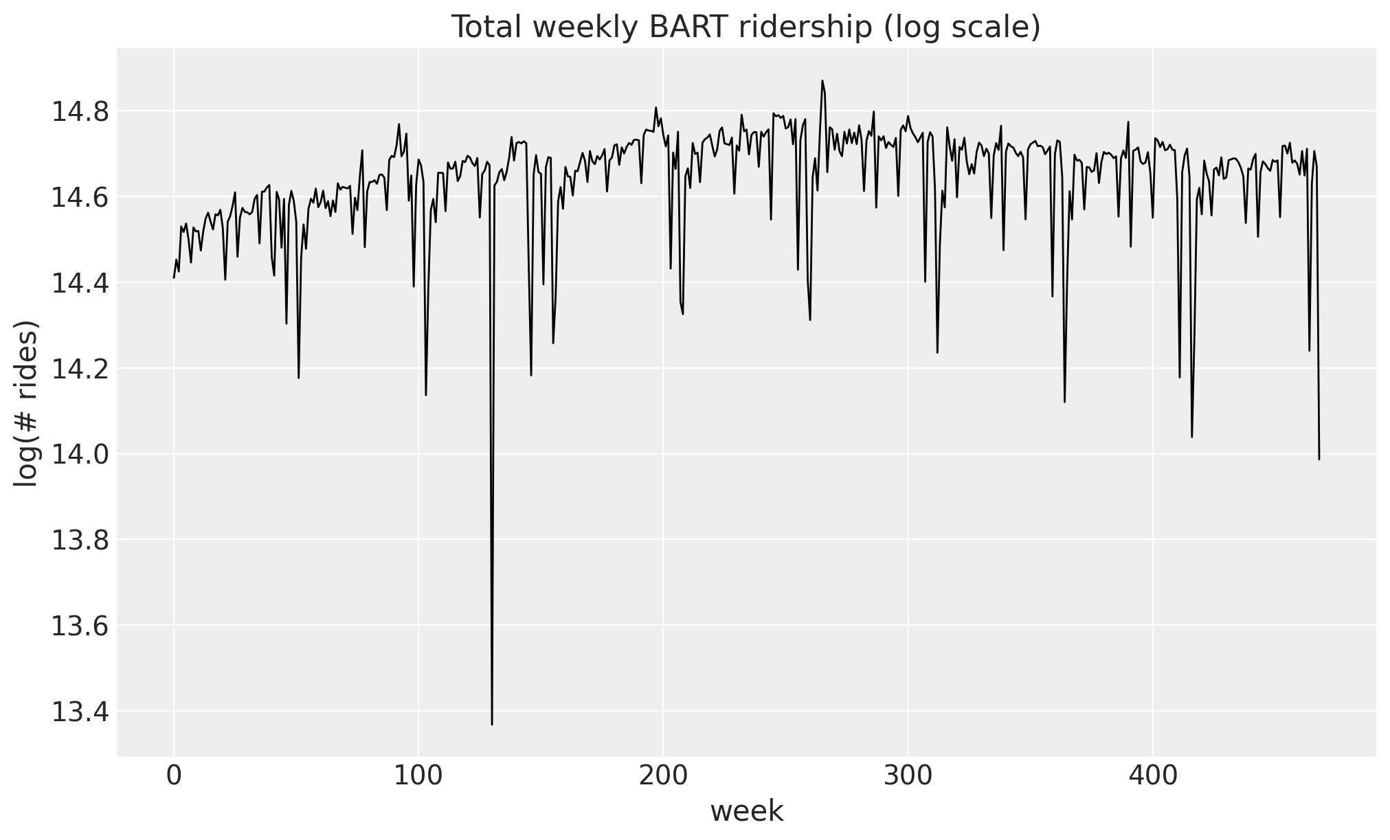
We work with total **weekly** BART ridership: hourly counts summed over all origin-destination pairs and aggregated into non-overlapping weeks. The series grows roughly multiplicatively, so we model it on the log scale, where the trend and the seasonal swings are closer to additive. Throughout the package, time lives at axis `-2` and the observation dimension at axis `-1`, so a single series has shape `(weeks, 1)`.
In [2]:
``` python
data = load_bart_weekly() # (weeks, 1), log scale
duration = data.shape[0]
print("data shape:", data.shape)
fig, ax = plt.subplots()
ax.plot(np.asarray(data[:, 0]), color="black", lw=1)
ax.set(
title="Total weekly BART ridership (log scale)",
xlabel="week",
ylabel="log(# rides)",
);
```
data shape: (469, 1)
# Train-test split
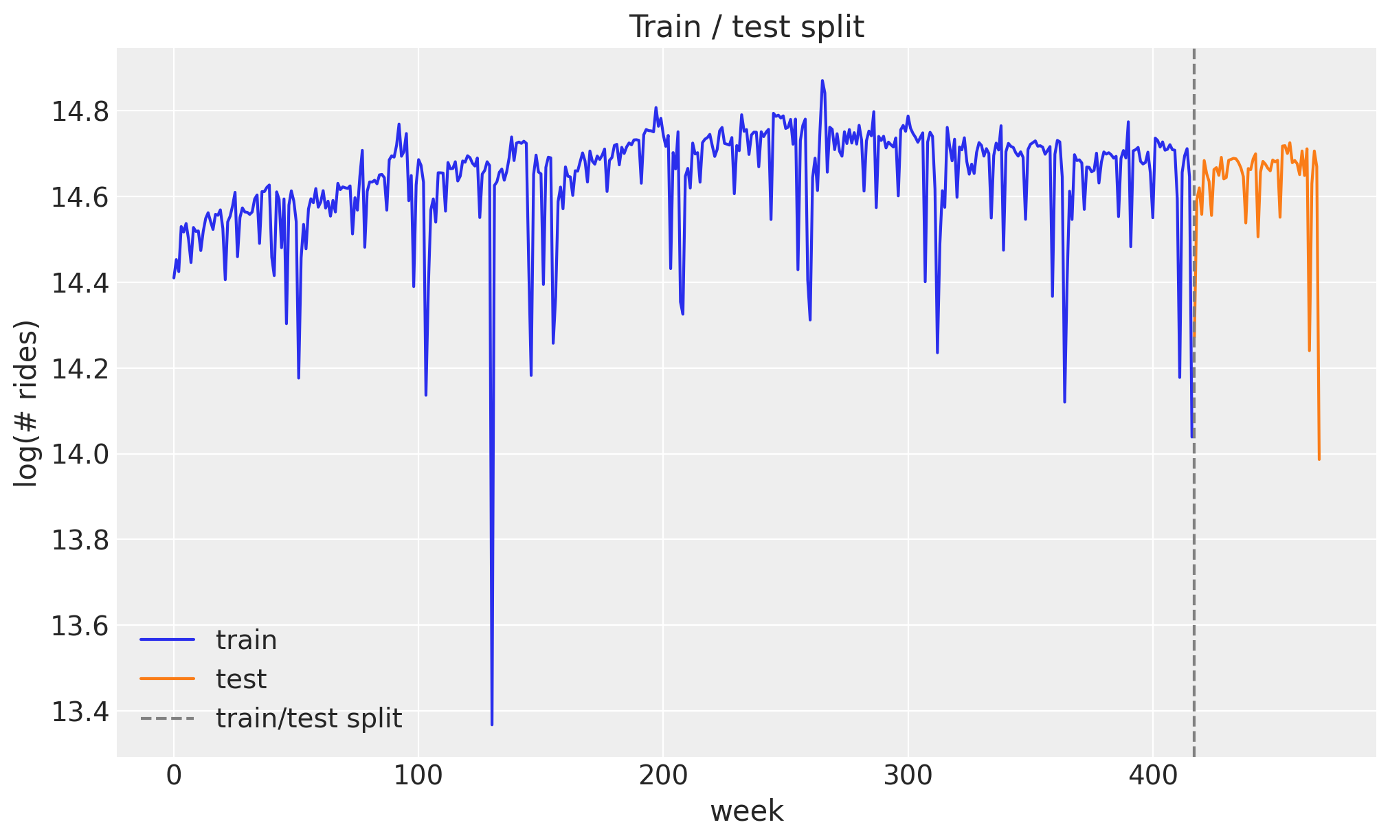
We hold out the last `52` weeks (one full year) as the test set and train on the preceding `417` weeks. Keeping a whole year out means the test window covers a complete seasonal cycle, which is exactly where a seasonal model can over- or under-fit.
In [3]:
``` python
T0 = 0
T2 = duration # 469
T1 = T2 - 52 # 417: train / test split
y_train = data[T0:T1]
y_test = data[T1:T2]
time = np.arange(T2)
time_train = time[T0:T1]
time_test = time[T1:T2]
print("train:", y_train.shape, "test:", y_test.shape)
fig, ax = plt.subplots()
ax.plot(time_train, np.asarray(y_train[:, 0]), color="C0", label="train")
ax.plot(time_test, np.asarray(y_test[:, 0]), color="C1", label="test")
ax.axvline(T1, color="gray", ls="--", label="train/test split")
ax.legend()
ax.set(title="Train / test split", xlabel="week", ylabel="log(# rides)");
```
train: (417, 1) test: (52, 1)
# Seasonal features
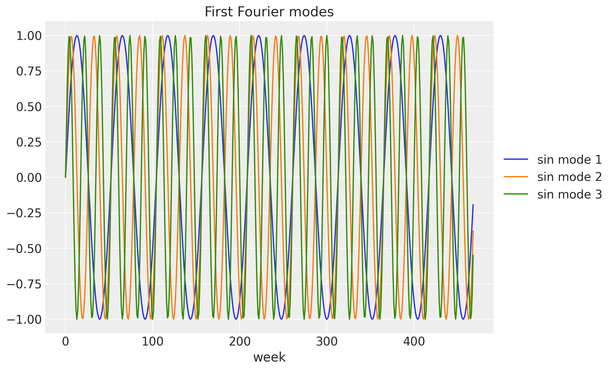
To capture the annual cycle we use a **Fourier** design matrix: `26` harmonics (so `52` sine and cosine columns) at a period of `365.25 / 7` weeks. Each harmonic is a sine/cosine pair at a multiple of the base frequency, and a weighted sum of them can approximate any smooth periodic shape. This spans the same subspace as the blog's `periodic_features`, so paired with the `Normal(0, 0.1)` weight prior the regression is equivalent. The plot below shows the first few low-frequency modes.
In [4]:
``` python
num_terms = 26
covariates = fourier_features(duration, period=365.25 / 7, num_terms=num_terms)
covariates_train = covariates[T0:T1]
print("covariates shape:", covariates.shape)
fig, ax = plt.subplots()
for k in range(3):
ax.plot(np.asarray(covariates[:, k]), label=f"sin mode {k + 1}")
ax.legend(loc="center left", bbox_to_anchor=(1, 0.5))
ax.set(title="First Fourier modes", xlabel="week");
```
covariates shape: (469, 52)
# Model specification
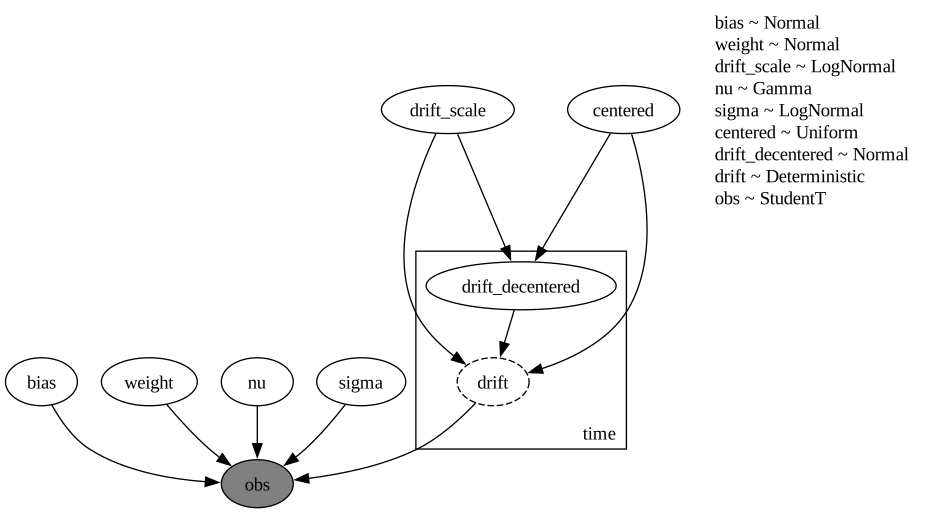
The idea is a *local level model with seasonality*. The mean has three parts: a global `bias`, a random-walk level \ell_t that lets the baseline drift slowly over time, and a Fourier regression for the annual cycle. The level moves by small Gaussian increments (the `drift`), so it can follow long-term changes without being told their shape in advance. For the likelihood we use a Student-T instead of a Normal: its heavy tails make the model robust to the occasional outlier week.
\begin{align\*} \mu_t & = \text{bias} + \ell_t + w^\top x_t, \\ \ell_t & = \ell\_{t-1} + \delta_t, \\ \delta_t & \sim \text{Normal}(0, \sigma\_\text{drift}), \\ y_t & \sim \text{StudentT}(\nu, \mu_t, \sigma). \end{align\*}
We subclass [ForecastingModel](../../../reference/forecaster.ForecastingModel.md#numpyro_forecast.forecaster.ForecastingModel) and write the generative story in [model](../../../reference/forecaster.ForecastingModel.md#numpyro_forecast.forecaster.ForecastingModel.model). The level is the cumulative sum of `drift`, which we sample with `self.time_series(...)` (the package's equivalent of the blog's `scan` over time). The single call to `self.predict(...)` registers the zero-centered Student-T noise around the predicted mean, and it is also what wires up the train-vs-forecast machinery: in-sample steps are observed, while the forecast horizon is drawn from separate `_future` latent sites so the variational guide never changes shape. Finally, a `LocScaleReparam` on the drift switches between centered and non-centered parameterizations, which helps the SVI geometry quite a lot.
In [5]:
``` python
class UnivariateForecaster(ForecastingModel):
"""Local level + Fourier regression with Student-T observations."""
def model(self, zero_data: Array | None, covariates: Array) -> None:
"""Define the univariate forecasting model."""
num_features = covariates.shape[-1]
bias = numpyro.sample("bias", dist.Normal(0.0, 10.0))
weight = numpyro.sample("weight", dist.Normal(0.0, 0.1).expand([num_features]).to_event(1))
drift_scale = numpyro.sample("drift_scale", dist.LogNormal(-20.0, 5.0))
nu = numpyro.sample("nu", dist.Gamma(10.0, 2.0))
sigma = numpyro.sample("sigma", dist.LogNormal(-5.0, 5.0))
centered = numpyro.sample("centered", dist.Uniform(0.0, 1.0))
drift = self.time_series(
"drift",
lambda: dist.Normal(0.0, drift_scale),
reparam=LocScaleReparam(centered=centered),
)
level = jnp.cumsum(drift, axis=-2)
regression = (weight * covariates).sum(axis=-1, keepdims=True)
prediction = level + bias + regression
self.predict(dist.StudentT(df=nu, loc=0.0, scale=sigma), prediction)
```
Let's visualize the model:
In [6]:
``` python
numpyro.render_model(
UnivariateForecaster(),
model_args=(covariates_train, y_train),
render_distributions=True,
)
```
# Prior predictive checks
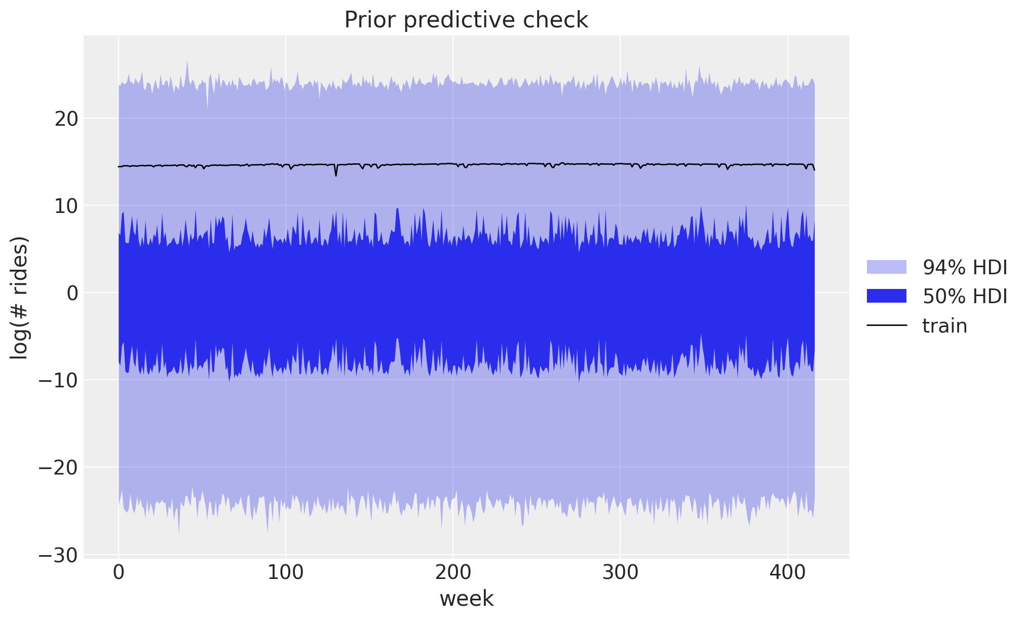
As usual (highly recommended!), we look at the prior predictive before fitting anything. We draw from the prior over the training window (`data=None`, so the horizon is zero and the `obs` site spans the train period) and plot the 50\\ and 94\\ HDI bands against the training series with ArviZ `plot_lm`. The priors are not very informative, but the implied ranges sit comfortably around the data, which is what we want.
In [7]:
``` python
prior_predictive = Predictive(UnivariateForecaster(), num_samples=2_000, return_sites=["obs"])
rng_key, rng_subkey = random.split(rng_key)
prior_obs = prior_predictive(rng_subkey, covariates_train)["obs"][..., 0]
idata_prior = az.from_dict(
{
"prior_predictive": {"obs": np.asarray(prior_obs)[None]},
"observed_data": {"obs": np.asarray(y_train[:, 0])},
"constant_data": {"week": time_train.astype(float)},
},
coords={"time": time_train.astype(float)},
dims={"obs": ["time"], "week": ["time"]},
)
pc = az.plot_lm(
idata_prior,
y="obs",
x="week",
group="prior_predictive",
ci_kind="hdi",
ci_prob=(0.5, 0.94),
smooth=False,
visuals={
"ci_band": {"color": "C0"},
"observed_scatter": False,
"pe_line": False,
},
figure_kwargs={"figsize": (10, 6)},
)
ax = pc.viz["figure"].item().axes[0]
bands = pc.viz["ci_band"]["week"]
band_94, band_50 = bands.sel(prob=0.94).item(), bands.sel(prob=0.5).item()
band_94.set_label(r"$94\%$ HDI")
band_50.set_label(r"$50\%$ HDI")
(train_line,) = ax.plot(time_train, np.asarray(y_train[:, 0]), color="black", lw=1, label="train")
ax.legend(handles=[band_94, band_50, train_line], loc="center left", bbox_to_anchor=(1, 0.5))
ax.set(title="Prior predictive check", ylabel="log(# rides)");
```
# Inference with SVI
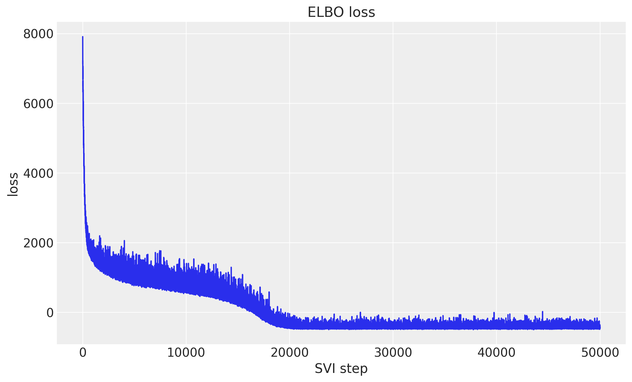
We fit the model with stochastic variational inference. Passing the model and data to [Forecaster](../../../reference/forecaster.Forecaster.md#numpyro_forecast.forecaster.Forecaster) runs SVI under the hood (an `AutoNormal` guide with `Adam`) and stores the fitted `guide`, `params` and the ELBO `losses`. The loss curve should decrease and flatten out, a quick sanity check that the optimization converged.
In [8]:
``` python
rng_key, rng_subkey = random.split(rng_key)
model = UnivariateForecaster()
forecaster = Forecaster(
rng_subkey,
model,
y_train,
covariates_train,
optim=Adam(step_size=0.005),
num_steps=50_000,
)
fig, ax = plt.subplots()
ax.plot(forecaster.losses)
ax.set(title="ELBO loss", xlabel="SVI step", ylabel="loss");
```
# Posterior predictive check
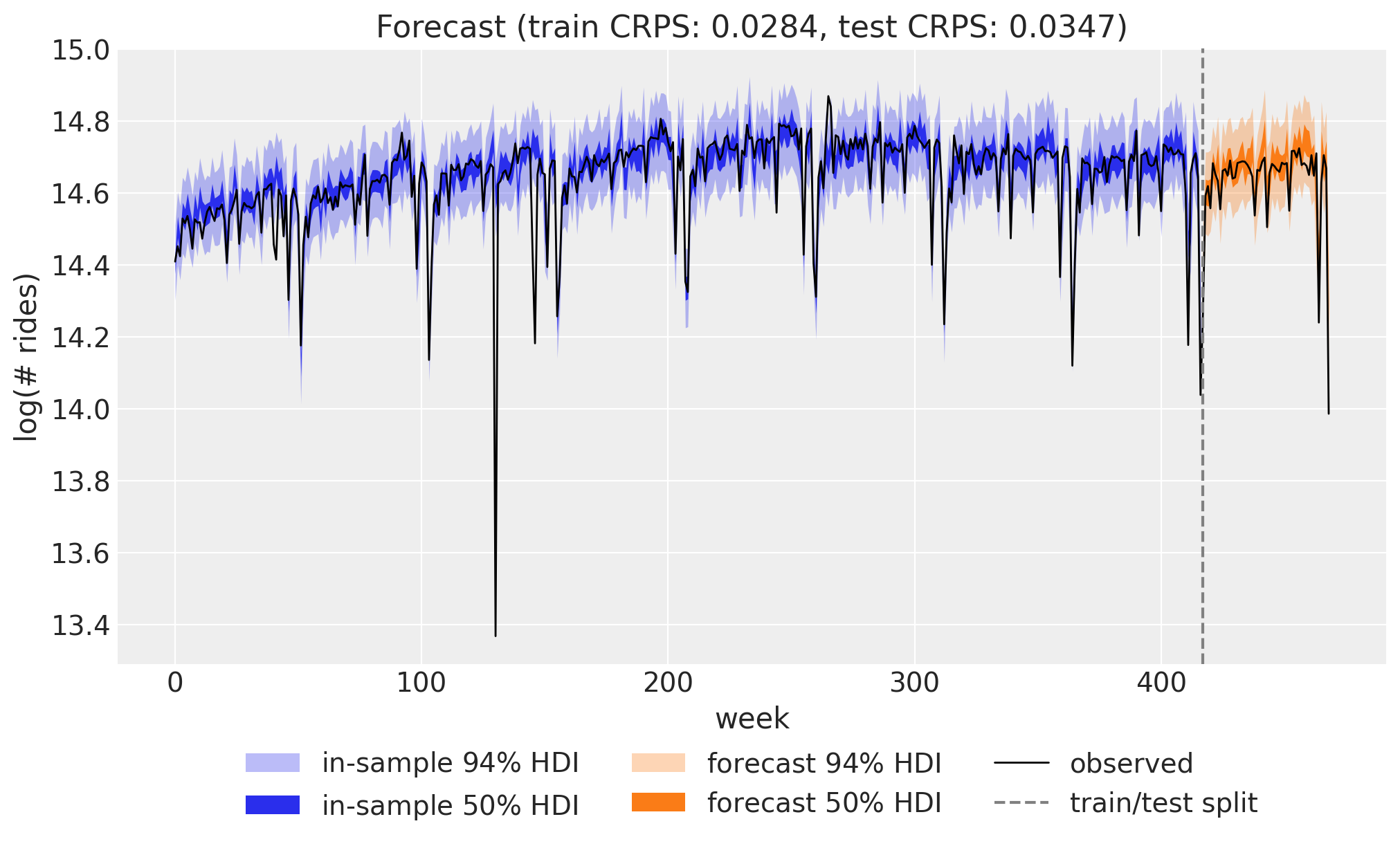
We now look at two things. First the **in-sample** posterior predictive over the training window: here the horizon is zero, so the guide is not resized and we just sample the `obs` site. Then the **forecast** over the test horizon with `forecaster(...)`, which continues the level from its inferred endpoint and draws the future random-walk increments from the prior.
To score both we use the **continuous ranked probability score** (CRPS), a proper scoring rule that compares a single ground-truth value to the whole forecast distribution rather than just a point estimate. It rewards forecasts that are both sharp and calibrated, and lower is better.
In [9]:
``` python
rng_key, key_pp, key_fc = random.split(rng_key, 3)
# In-sample posterior predictive over the training window.
train_pp = forecaster.predict_in_sample(key_pp, covariates_train, num_samples=5_000)
# Forecast over the test horizon.
forecast = forecaster(key_fc, y_train, covariates, num_samples=5_000)
crps_train = eval_crps(train_pp, y_train)
crps_test = eval_crps(forecast, y_test)
print(f"Train CRPS: {crps_train:.4f}")
print(f"Test CRPS: {crps_test:.4f}")
print(f"Test 50% coverage: {eval_coverage(forecast, y_test, alpha=0.5):.2f} (nominal 0.50)")
print(f"Test 94% coverage: {eval_coverage(forecast, y_test, alpha=0.94):.2f} (nominal 0.94)")
```
Train CRPS: 0.0284
Test CRPS: 0.0347
Test 50% coverage: 0.63 (nominal 0.50)
Test 94% coverage: 0.92 (nominal 0.94)
# Forecast visualization
The combined view puts everything together: the in-sample posterior predictive (blue) and the forecast over the held-out year (orange), each with 50\\ and 94\\ HDI bands, against the observed series. The forecast tracks the seasonal pattern and the uncertainty widens into the future, as it should.
In [10]:
``` python
train_obs = train_pp[..., 0]
forecast_obs = forecast[..., 0]
idata_train = az.from_dict(
{
"posterior_predictive": {"obs": np.asarray(train_obs)[None]},
"observed_data": {"obs": np.asarray(y_train[:, 0])},
"constant_data": {"week": time_train.astype(float)},
},
coords={"time": time_train.astype(float)},
dims={"obs": ["time"], "week": ["time"]},
)
idata_test = az.from_dict(
{
"posterior_predictive": {"obs": np.asarray(forecast_obs)[None]},
"observed_data": {"obs": np.asarray(y_test[:, 0])},
"constant_data": {"week": time_test.astype(float)},
},
coords={"time": time_test.astype(float)},
dims={"obs": ["time"], "week": ["time"]},
)
pc = az.plot_lm(
idata_train,
y="obs",
x="week",
ci_kind="hdi",
ci_prob=(0.5, 0.94),
smooth=False,
visuals={"ci_band": {"color": "C0"}, "observed_scatter": False, "pe_line": False},
figure_kwargs={"figsize": (10, 6)},
)
train_bands = pc.viz["ci_band"]["week"]
band_train_94 = train_bands.sel(prob=0.94).item()
band_train_50 = train_bands.sel(prob=0.5).item()
az.plot_lm(
idata_test,
y="obs",
x="week",
plot_collection=pc,
ci_kind="hdi",
ci_prob=(0.5, 0.94),
smooth=False,
visuals={"ci_band": {"color": "C1"}, "observed_scatter": False, "pe_line": False},
)
test_bands = pc.viz["ci_band"]["week"]
band_test_94 = test_bands.sel(prob=0.94).item()
band_test_50 = test_bands.sel(prob=0.5).item()
ax = pc.viz["figure"].item().axes[0]
band_train_94.set_label(r"in-sample $94\%$ HDI")
band_train_50.set_label(r"in-sample $50\%$ HDI")
band_test_94.set_label(r"forecast $94\%$ HDI")
band_test_50.set_label(r"forecast $50\%$ HDI")
(obs_line,) = ax.plot(time, np.asarray(data[:, 0]), color="black", lw=1, label="observed")
split_line = ax.axvline(T1, color="gray", ls="--", label="train/test split")
ax.legend(
handles=[band_train_94, band_train_50, band_test_94, band_test_50, obs_line, split_line],
loc="upper center",
bbox_to_anchor=(0.5, -0.1),
ncol=3,
)
ax.set(
title=f"Forecast (train CRPS: {crps_train:.4f}, test CRPS: {crps_test:.4f})",
ylabel="log(# rides)",
);
```
# Rolling-origin backtesting
A single train/test split tells us how the model did on one held-out year. A more honest picture of generalization comes from *rolling-origin* backtesting: we repeatedly move the train/test boundary forward, refit, and forecast the next window, so every later part of the series is scored out-of-sample exactly once. `numpyro_forecast.backtest` runs this loop on the full series for us, refitting a fresh `UnivariateForecaster` per fold.
[backtest](../../../reference/evaluate.backtest.md#numpyro_forecast.evaluate.backtest) offers two windowing strategies through its `window_type` argument. An **expanding** window (the default) trains each fold on all history up to its split point, so the training set grows fold by fold. A **rolling** window instead holds the training length fixed at `train_window` and slides it forward, so every fold sees the same number of most-recent observations while older data drops off the back. We walk through the expanding window first, then contrast the two directly at the end of this section.
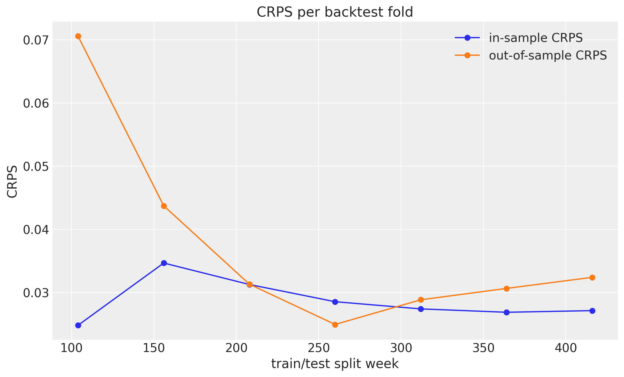
We use an expanding window: each fold trains on everything up to its split point and forecasts the next `52` weeks (`test_window=52`), stepping forward a full year at a time (`stride=52`) so the folds do not overlap and the forecast overlay stays readable. The first `min_train_window=104` weeks (two years) seed the initial training window, matching Pyro's tutorial. With `eval_train=True` we also score the in-sample posterior predictive of each fold with the same CRPS metric, and `keep_predictions=True` retains each fold's out-of-sample forecast samples so we can plot them. Both options default to off, keeping the default [backtest](../../../reference/evaluate.backtest.md#numpyro_forecast.evaluate.backtest) API faithful to Pyro.
One practical point: because every fold is refit from scratch, each one needs enough optimization to converge. We give SVI `num_steps=50_000` per fold (the same budget as the main fit) so that the larger expanding windows are fit just as well as the small early ones, which keeps the inferred drift volatility stable and the per-fold scores comparable. With too small a budget the later windows would be under-fit, inflating `drift_scale` so that both the forecast bands and the in-sample CRPS grow spuriously with window length.
In [11]:
``` python
num_backtest_samples = 2_000
metrics = {
"crps": eval_crps,
"coverage_50": partial(eval_coverage, alpha=0.5),
"coverage_94": partial(eval_coverage, alpha=0.94),
}
rng_key, rng_subkey = random.split(rng_key)
results = backtest(
rng_subkey,
data, # full dataset, no train/test split
covariates, # full covariates
UnivariateForecaster,
metrics=metrics,
test_window=52, # 1-year horizon per fold
stride=52, # non-overlapping folds for a clean plot_lm panel
min_train_window=104, # 2 years before the first fold, matching Pyro's start
num_samples=num_backtest_samples,
eval_train=True,
keep_predictions=True,
forecaster_options={"optim": Adam(step_size=0.005), "num_steps": 50_000},
)
split_weeks = [r.t1 for r in results]
insample_crps = [r.train_metrics["crps"] for r in results]
oos_crps = [r.metrics["crps"] for r in results]
oos_cov_50 = [r.metrics["coverage_50"] for r in results]
oos_cov_94 = [r.metrics["coverage_94"] for r in results]
print(f"folds: {len(results)}")
print(f"mean in-sample CRPS: {np.mean(insample_crps):.4f}")
print(f"mean out-of-sample CRPS: {np.mean(oos_crps):.4f}")
print(f"mean out-of-sample 50% coverage: {np.mean(oos_cov_50):.2f} (nominal 0.50)")
print(f"mean out-of-sample 94% coverage: {np.mean(oos_cov_94):.2f} (nominal 0.94)")
```
folds: 7
mean in-sample CRPS: 0.0287
mean out-of-sample CRPS: 0.0375
mean out-of-sample 50% coverage: 0.57 (nominal 0.50)
mean out-of-sample 94% coverage: 0.95 (nominal 0.94)
## Rolling forecasts
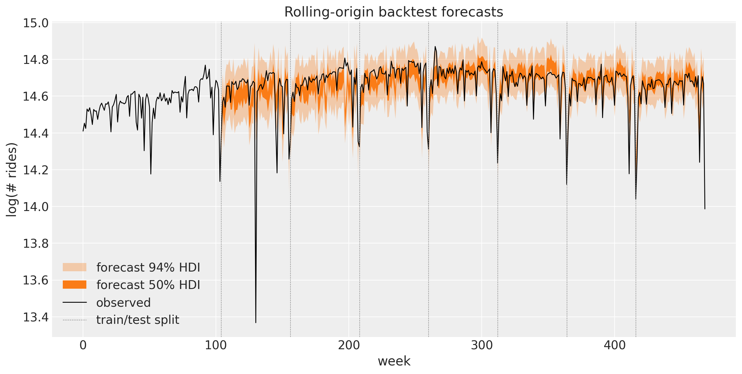
Overlaying every fold's out-of-sample forecast (orange 50\\ and 94\\ HDI bands) on the full observed series gives the rolling-origin view: each band picks up where the previous fold's training data ended, so together they trace a continuous one-year-ahead forecast across the second half of the series. The dashed lines mark the successive train/test splits.
In [12]:
``` python
pc = None
for r in results:
prediction = r.prediction
if prediction is None: # keep_predictions=True guarantees this never triggers
continue
weeks = time[r.t1 : r.t2].astype(float)
idata = az.from_dict(
{
"posterior_predictive": {"obs": np.asarray(prediction[..., 0])[None]},
"observed_data": {"obs": np.asarray(data[r.t1 : r.t2, 0])},
"constant_data": {"week": weeks},
},
coords={"time": weeks},
dims={"obs": ["time"], "week": ["time"]},
)
if pc is None:
pc = az.plot_lm(
idata,
y="obs",
x="week",
ci_kind="hdi",
ci_prob=(0.5, 0.94),
smooth=False,
visuals={"ci_band": {"color": "C1"}, "observed_scatter": False, "pe_line": False},
figure_kwargs={"figsize": (12, 6)},
)
bands = pc.viz["ci_band"]["week"]
band_94, band_50 = bands.sel(prob=0.94).item(), bands.sel(prob=0.5).item()
else:
az.plot_lm(
idata,
y="obs",
x="week",
plot_collection=pc,
ci_kind="hdi",
ci_prob=(0.5, 0.94),
smooth=False,
visuals={"ci_band": {"color": "C1"}, "observed_scatter": False, "pe_line": False},
)
if pc is None:
msg = "no folds were plotted"
raise ValueError(msg)
ax = pc.viz["figure"].item().axes[0]
band_94.set_label(r"forecast $94\%$ HDI")
band_50.set_label(r"forecast $50\%$ HDI")
(obs_line,) = ax.plot(time, np.asarray(data[:, 0]), color="black", lw=1, label="observed")
split_lines = [
ax.axvline(r.t1, color="gray", ls="--", lw=0.5, label="train/test split") for r in results
]
ax.set(title="Rolling-origin backtest forecasts", ylabel="log(# rides)")
ax.legend(handles=[band_94, band_50, obs_line, split_lines[0]], loc="lower left");
```
Within each fold the band fans out gently from its train/test split toward the right. That is the random-walk level diffusing: the level is a cumulative sum of drift increments (`level = jnp.cumsum(drift, axis=-2)`), and over the forecast horizon those future increments are drawn from the prior, so the predictive standard deviation grows like the square root of the horizon. The seasonal Fourier term is periodic and the Student-T observation noise is roughly constant, so this within-fold growth is dominated by the level diffusing. It is irreducible: more training data cannot make next year's random increments knowable.
Across folds the bands reset at each dashed split, where the model is refit and re-conditioned on all data up to that point, and their width stays stable from fold to fold. Each fold is fit with `num_steps=50_000` (the same budget as the main fit), so every expanding window converges and the inferred drift volatility is consistent. The bands therefore do not balloon as the series lengthens; under-training would leave the larger windows under-fit, inflate `drift_scale`, and widen the later folds spuriously.
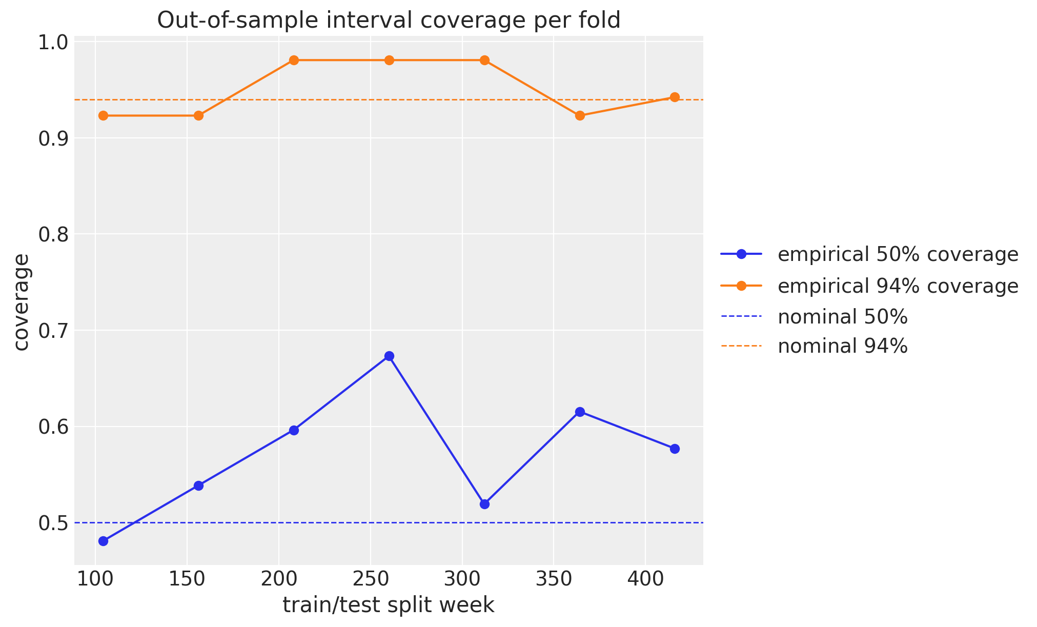
The fit looks well calibrated, and the coverage plot further below makes that claim precise: the observed series stays inside the 94% band almost everywhere and inside the 50% band roughly half the time, close to the nominal levels. The sharp downward holiday spikes occasionally pierce the lower band, and that is by design: the heavy-tailed Student-T likelihood treats them as outliers rather than widening the whole band to swallow them.
## CRPS per fold
The per-fold CRPS shows the model generalizing better as it sees more history. The out-of-sample score is highest for the first, data-starved fold (trained on just the initial two years) and falls steeply as the expanding window grows, then flattens out near the in-sample level: more training data buys a sharper, better-calibrated one-year-ahead forecast, exactly as we would hope. The in-sample CRPS stays low and roughly flat across folds, because with `num_steps=50_000` each fold converges regardless of window length, so the fit quality does not drift.
The train-versus-test gap is therefore widest early, when data is scarce, and closes as history accumulates (the two curves even cross near the middle of the series). That closing gap is the healthy signature of a model whose generalization improves with more data, rather than an under-fit whose error would instead grow with window length. If you shrink `num_steps` you will see that healthy pattern break: both curves climb with the window as the larger folds stop converging.
In [13]:
``` python
fig, ax = plt.subplots()
ax.plot(split_weeks, insample_crps, "o-", color="C0", label="in-sample CRPS")
ax.plot(split_weeks, oos_crps, "o-", color="C1", label="out-of-sample CRPS")
ax.legend()
ax.set(xlabel="train/test split week", ylabel="CRPS", title="CRPS per backtest fold");
```
## Forecast calibration
CRPS rewards sharp *and* calibrated forecasts but does not separate the two, so "the forecasts look calibrated" deserves its own number. We score the empirical **coverage** of each fold's out-of-sample bands: the fraction of held-out weeks that actually fall inside the central 50\\ and 94\\ prediction intervals. A well-calibrated forecast covers close to its nominal level, so the points should track the dashed reference lines. Points above mean the bands are too wide (under-confident); points below mean they are too narrow (over-confident). This is the quantitative version of the "stays inside the bands" eyeball check from the rolling-forecast plot.
A small caveat: [eval_coverage](../../../reference/evaluate.eval_coverage.md#numpyro_forecast.evaluate.eval_coverage) measures coverage of the central quantile interval, while the plotted bands are arviz HDI. For the near-symmetric Student-T posterior predictive here the two nearly coincide, so this is a faithful check of the bands shown above.
In [14]:
``` python
fig, ax = plt.subplots()
ax.plot(split_weeks, oos_cov_50, "o-", color="C0", label=r"empirical $50\%$ coverage")
ax.plot(split_weeks, oos_cov_94, "o-", color="C1", label=r"empirical $94\%$ coverage")
ax.axhline(0.5, color="C0", ls="--", lw=1, label=r"nominal $50\%$")
ax.axhline(0.94, color="C1", ls="--", lw=1, label=r"nominal $94\%$")
ax.legend(loc="center left", bbox_to_anchor=(1, 0.5))
ax.set(
xlabel="train/test split week",
ylabel="coverage",
title="Out-of-sample interval coverage per fold",
);
```
## Expanding vs rolling windows
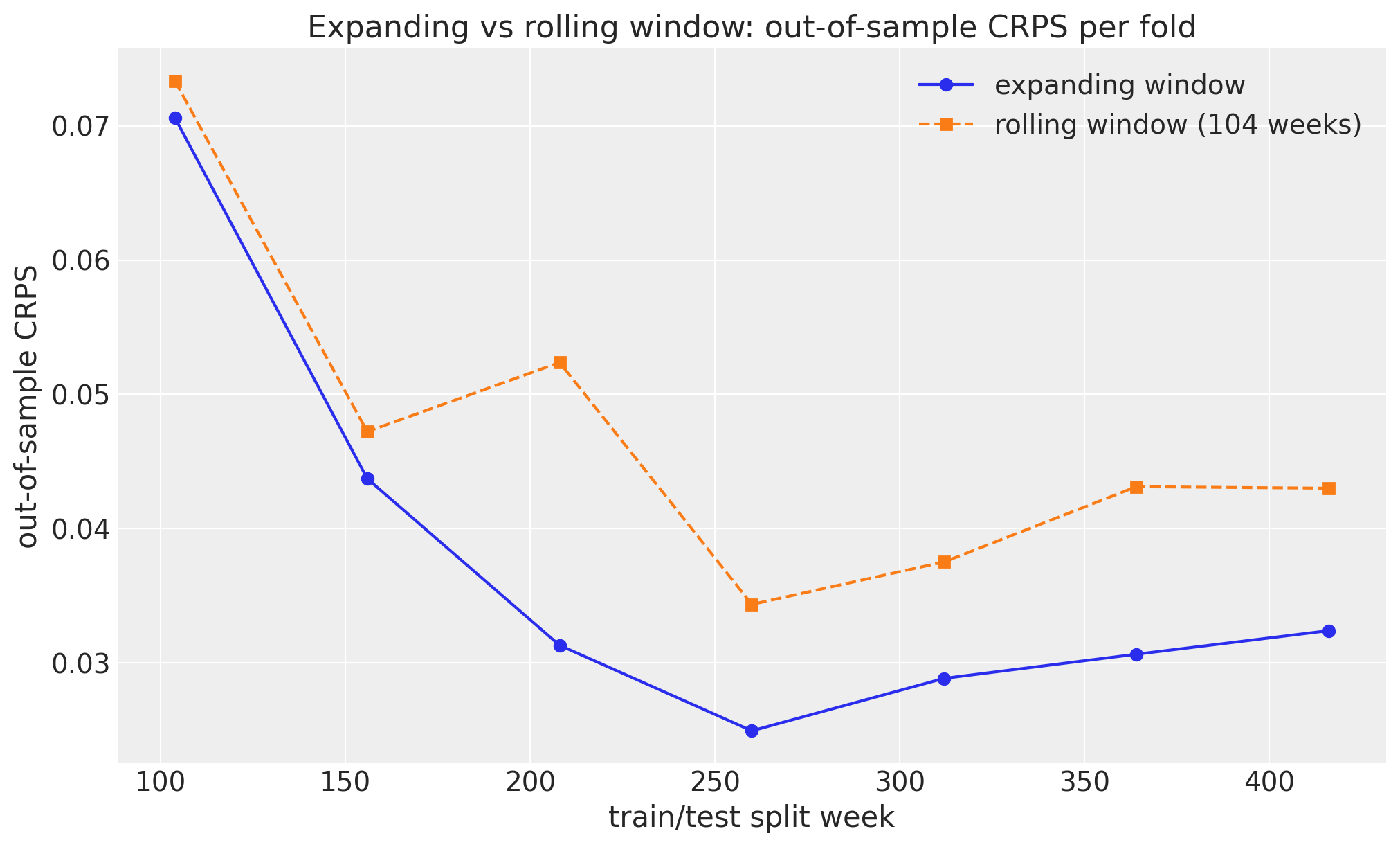
The run above expanded the training window fold by fold. Switching to a **rolling** window takes a single argument, `window_type="rolling"`, plus a fixed `train_window`. We rerun the same backtest with a `104`-week (two-year) rolling window, matching the expanding run's seed so the two share identical split points, horizon, stride, sample count, and SVI budget. The only thing that changes is whether each fold keeps the older history or drops it.
In [15]:
``` python
rng_key, rng_subkey = random.split(rng_key)
rolling_results = backtest(
rng_subkey,
data,
covariates,
UnivariateForecaster,
metrics=metrics,
window_type="rolling", # fixed-size training window instead of expanding
train_window=104, # 2 years, matching the expanding seed so the split points line up
test_window=52, # 1-year horizon per fold, as before
stride=52, # same non-overlapping folds
num_samples=num_backtest_samples,
forecaster_options={"optim": Adam(step_size=0.005), "num_steps": 50_000},
)
rolling_oos_crps = [r.metrics["crps"] for r in rolling_results]
print(f"expanding folds: {len(results)} | rolling folds: {len(rolling_results)}")
print(f"expanding mean out-of-sample CRPS: {np.mean(oos_crps):.4f}")
print(f"rolling mean out-of-sample CRPS: {np.mean(rolling_oos_crps):.4f}")
for wk, exp_c, roll_c in zip(split_weeks, oos_crps, rolling_oos_crps, strict=True):
print(f" split week {wk:>3}: expanding {exp_c:.4f} rolling {roll_c:.4f}")
```
expanding folds: 7 | rolling folds: 7
expanding mean out-of-sample CRPS: 0.0375
rolling mean out-of-sample CRPS: 0.0473
split week 104: expanding 0.0706 rolling 0.0733
split week 156: expanding 0.0437 rolling 0.0472
split week 208: expanding 0.0313 rolling 0.0524
split week 260: expanding 0.0250 rolling 0.0344
split week 312: expanding 0.0289 rolling 0.0375
split week 364: expanding 0.0307 rolling 0.0431
split week 416: expanding 0.0324 rolling 0.0430
Both strategies train each fold on the same fixed `104`-week window at the first split, then diverge: the expanding window keeps every additional year while the rolling window always discards all but the most recent two.
In [16]:
``` python
fig, ax = plt.subplots()
ax.plot(split_weeks, oos_crps, "o-", color="C0", label="expanding window")
ax.plot(split_weeks, rolling_oos_crps, "s--", color="C1", label="rolling window (104 weeks)")
ax.legend()
ax.set(
xlabel="train/test split week",
ylabel="out-of-sample CRPS",
title="Expanding vs rolling window: out-of-sample CRPS per fold",
);
```
The mechanism behind the two curves is the random-walk level. Each forecast is anchored at the last observed level and fans out at a rate set by the inferred drift volatility `drift_scale`, which every fold estimates from its own training window. The expanding window estimates that volatility from all history and keeps sharpening it as data accumulates, so its out-of-sample CRPS falls steeply after the data-starved first fold and then settles near the in-sample floor. The rolling window only ever sees the most recent two years, so after its own early improvement it plateaus at a higher, noisier level: it keeps discarding the extra history that the expanding window compounds.
Here the expanding window is the clear winner: it scores a lower out-of-sample CRPS on every fold (mean `0.0375` versus `0.0473`), and the two are closest only at the first split, where they happen to train on the same two years, before the gap opens up. That is what we should expect on this BART series, where the trend and seasonality are stable and old observations stay informative, so throwing them away can only hurt. The rolling window earns its keep on a different kind of series, one with structural breaks or slow regime drift, where distant history is misleading rather than helpful and a fixed recency focus keeps the forecast adapting, at a bounded, constant fitting cost per fold. `window_type` lets you encode whichever assumption matches your data without touching anything else in the backtest.
## Vectorized rolling backtest
The rolling loop above refits one fold at a time, so each fold pays its own SVI compilation and Python-loop overhead. Because every fold shares the same model, guide, and window sizes, [backtest_vectorized](../../../reference/evaluate.backtest_vectorized.md#numpyro_forecast.evaluate.backtest_vectorized) can instead fit **all folds in a single vmapped SVI run**: model, guide, and optimizer compile once, and the per-fold losses, forecasts, and metrics come out stacked along a leading window axis.
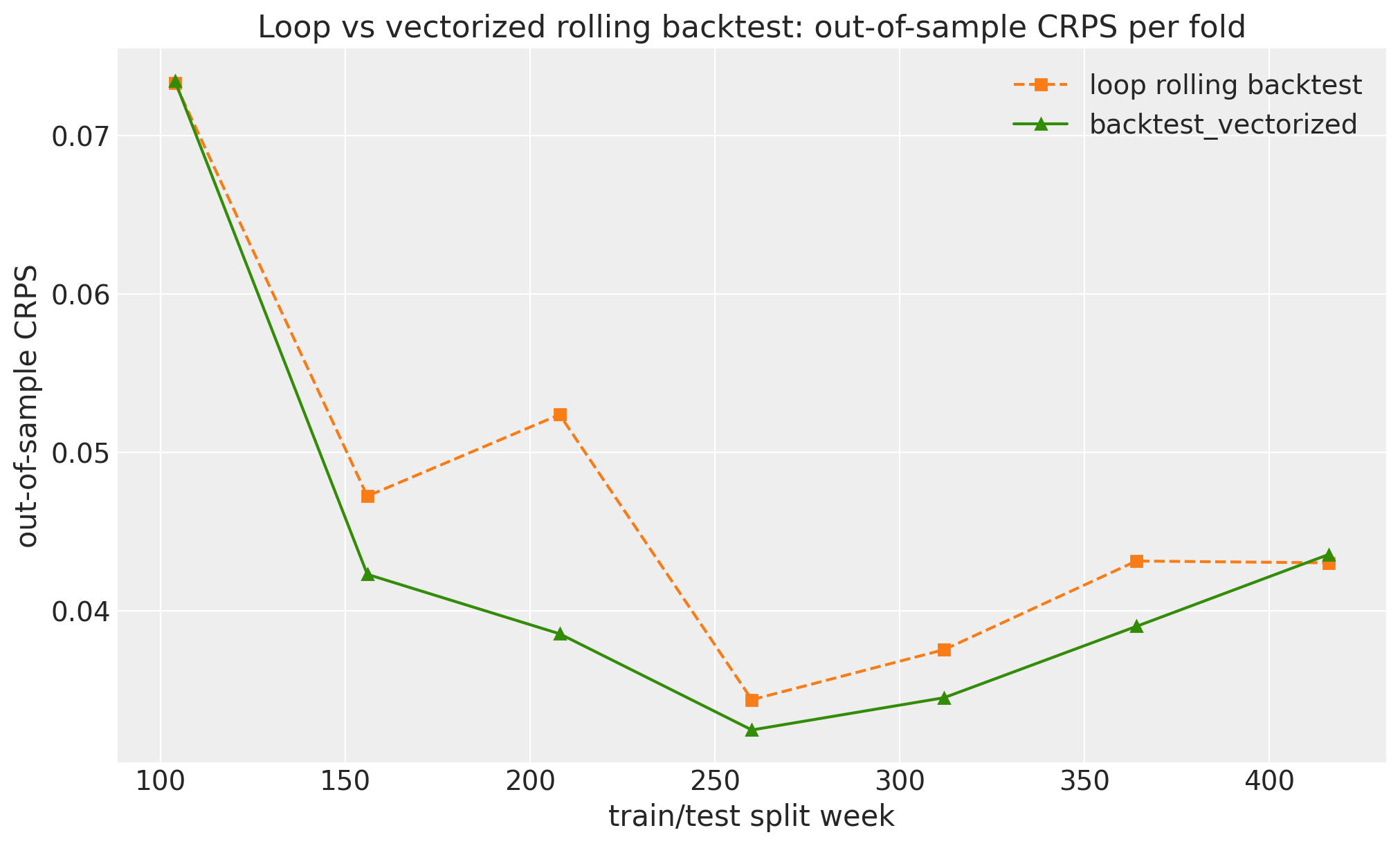
The `metrics` mapping needs no change at all. Metrics are pure JAX scalar kernels, so the partial-bound 50\\ and 94\\ coverage levels defined earlier are scored inside the same single fused computation, right alongside the default CRPS. The two backtests are estimator-equivalent but differ in PRNG stream layout, so the per-fold numbers agree statistically rather than bitwise.
In [17]:
``` python
rng_key, rng_subkey = random.split(rng_key)
start_seconds = perf_counter()
vectorized_results = backtest_vectorized(
rng_subkey,
data,
covariates,
UnivariateForecaster,
train_window=104, # same rolling configuration as the loop run above
test_window=52,
stride=52,
num_steps=50_000,
optim=Adam(step_size=0.005),
num_samples=num_backtest_samples,
metrics=metrics, # same custom mapping, including both partial-bound coverage levels
)
vectorized_seconds = perf_counter() - start_seconds
loop_seconds = sum(r.train_walltime + r.test_walltime for r in rolling_results)
vectorized_oos_crps = np.asarray(vectorized_results.metrics["crps"])
vectorized_cov_50 = float(vectorized_results.metrics["coverage_50"].mean())
vectorized_cov_94 = float(vectorized_results.metrics["coverage_94"].mean())
print(f"folds: {vectorized_results.t0.shape[0]} in one vmapped SVI fit")
print(
f"wall-clock: vectorized {vectorized_seconds:.1f}s (incl. compile)"
f" | loop {loop_seconds:.1f}s"
)
print(f"vectorized mean out-of-sample CRPS: {vectorized_oos_crps.mean():.4f}")
print(f"loop mean out-of-sample CRPS: {np.mean(rolling_oos_crps):.4f}")
print(f"vectorized mean 50% coverage: {vectorized_cov_50:.2f} (nominal 0.50)")
print(f"vectorized mean 94% coverage: {vectorized_cov_94:.2f} (nominal 0.94)")
```
folds: 7 in one vmapped SVI fit
wall-clock: vectorized 2.0s (incl. compile) | loop 19.2s
vectorized mean out-of-sample CRPS: 0.0434
loop mean out-of-sample CRPS: 0.0473
vectorized mean 50% coverage: 0.50 (nominal 0.50)
vectorized mean 94% coverage: 0.95 (nominal 0.94)
In [18]:
``` python
fig, ax = plt.subplots()
ax.plot(split_weeks, rolling_oos_crps, "s--", color="C1", label="loop rolling backtest")
ax.plot(split_weeks, vectorized_oos_crps, "^-", color="C2", label="backtest_vectorized")
ax.legend()
ax.set(
xlabel="train/test split week",
ylabel="out-of-sample CRPS",
title="Loop vs vectorized rolling backtest: out-of-sample CRPS per fold",
);
```
Both estimators tell the same story fold by fold, and the printed wall-clock numbers show what a single fused fit buys on this model; the vectorized advantage grows with the number of folds, since compilation is paid once rather than per fold. The trade-offs are spelled out in the [backtest_vectorized](../../../reference/evaluate.backtest_vectorized.md#numpyro_forecast.evaluate.backtest_vectorized) docstring: fixed-size rolling windows only, one shared model instance, an `AutoGuide`, and pure JAX metrics, which the coverage partials above already are.
# Functional API
Everything so far went through the object-oriented [ForecastingModel](../../../reference/forecaster.ForecastingModel.md#numpyro_forecast.forecaster.ForecastingModel), but that class is only a thin shim over a functional core in `numpyro_forecast.functional`. The same model can be written as a plain function `(Horizon, covariates) -> None` that calls the free functions [time_series](../../../reference/functional.models.time_series.md#numpyro_forecast.functional.models.time_series) and [predict](../../../reference/functional.models.predict.md#numpyro_forecast.functional.models.predict) (the exact counterparts of the `self.time_series(...)` and `self.predict(...)` methods used above). The [Horizon](../../../reference/functional.models.Horizon.md#numpyro_forecast.functional.models.Horizon) carries the train/forecast split that the class otherwise tracks as mutable state.
`forecasting_model(...)` then wraps that body into the standard `(covariates, data=None)` NumPyro model, so the result is a drop-in replacement for a `UnivariateForecaster()` instance: it works with [Forecaster](../../../reference/forecaster.Forecaster.md#numpyro_forecast.forecaster.Forecaster), `Predictive`, and [backtest](../../../reference/evaluate.backtest.md#numpyro_forecast.evaluate.backtest) just the same. We rewrite the model below and confirm the two are interchangeable.
In [19]:
``` python
def univariate_model(h: Horizon, covariates: Array) -> None:
"""Functional twin of ``UnivariateForecaster.model``."""
num_features = covariates.shape[-1]
bias = numpyro.sample("bias", dist.Normal(0.0, 10.0))
weight = numpyro.sample("weight", dist.Normal(0.0, 0.1).expand([num_features]).to_event(1))
drift_scale = numpyro.sample("drift_scale", dist.LogNormal(-20.0, 5.0))
nu = numpyro.sample("nu", dist.Gamma(10.0, 2.0))
sigma = numpyro.sample("sigma", dist.LogNormal(-5.0, 5.0))
centered = numpyro.sample("centered", dist.Uniform(0.0, 1.0))
drift = time_series(
h,
"drift",
lambda: dist.Normal(0.0, drift_scale),
reparam=LocScaleReparam(centered=centered),
)
level = jnp.cumsum(drift, axis=-2)
regression = (weight * covariates).sum(axis=-1, keepdims=True)
prediction = level + bias + regression
predict(h, dist.StudentT(df=nu, loc=0.0, scale=sigma), prediction)
functional_model = forecasting_model(univariate_model)
```
To check the two are the same model, we draw a prior forward sample from each with the **same** `rng_subkey` and compare the `obs` site. Since `obs` sits downstream of every latent, matching `obs` draws imply the whole forward computation matched.
In [20]:
``` python
rng_key, rng_subkey = random.split(rng_key)
oop_obs = Predictive(UnivariateForecaster(), num_samples=100, return_sites=["obs"])(
rng_subkey, covariates_train
)["obs"]
func_obs = Predictive(functional_model, num_samples=100, return_sites=["obs"])(
rng_subkey, covariates_train
)["obs"]
print("identical forward samples:", bool(jnp.array_equal(oop_obs, func_obs)))
print("max abs difference:", float(jnp.max(jnp.abs(oop_obs - func_obs))))
```
identical forward samples: True
max abs difference: 0.0
The forward samples are bit-identical (maximum difference `0.0`): both models issue the same sample statements in the same order, so the random-number stream lines up exactly. The object-oriented class and the functional model are fully interchangeable, and you can reach for whichever style fits the problem.
# Next steps
This local level model with seasonality is a solid baseline. From here a few directions are natural: add holiday or special-event effects (dummy variables or Gaussian bump functions) for days the smooth seasonal basis cannot capture, or move to many related series at once. The last of these is the subject of the two companion notebooks, [hierarchical forecasting I](hierarchical_forecasting_1.md) and [II](hierarchical_forecasting_2.md), which generalize this same model to a panel of BART stations. See also Pyro's original [forecasting tutorial](https://pyro.ai/examples/forecasting_i.html).
# References
- Orduz, J. [*Univariate time series forecasting with NumPyro*](https://juanitorduz.github.io/numpyro_forecasting-univariate/).
- Pyro. [*Forecasting I: Univariate, Heavy Tailed*](https://pyro.ai/examples/forecasting_i.html).