Scaling Probabilistic Models with Variational Inference

PyData Berlin 2025

Dr. Juan Orduz

Outline

• Motivating Examples

• Variational Inference in a Nutshell

• Toy Example: Parameter Recovery Gamma Distribution

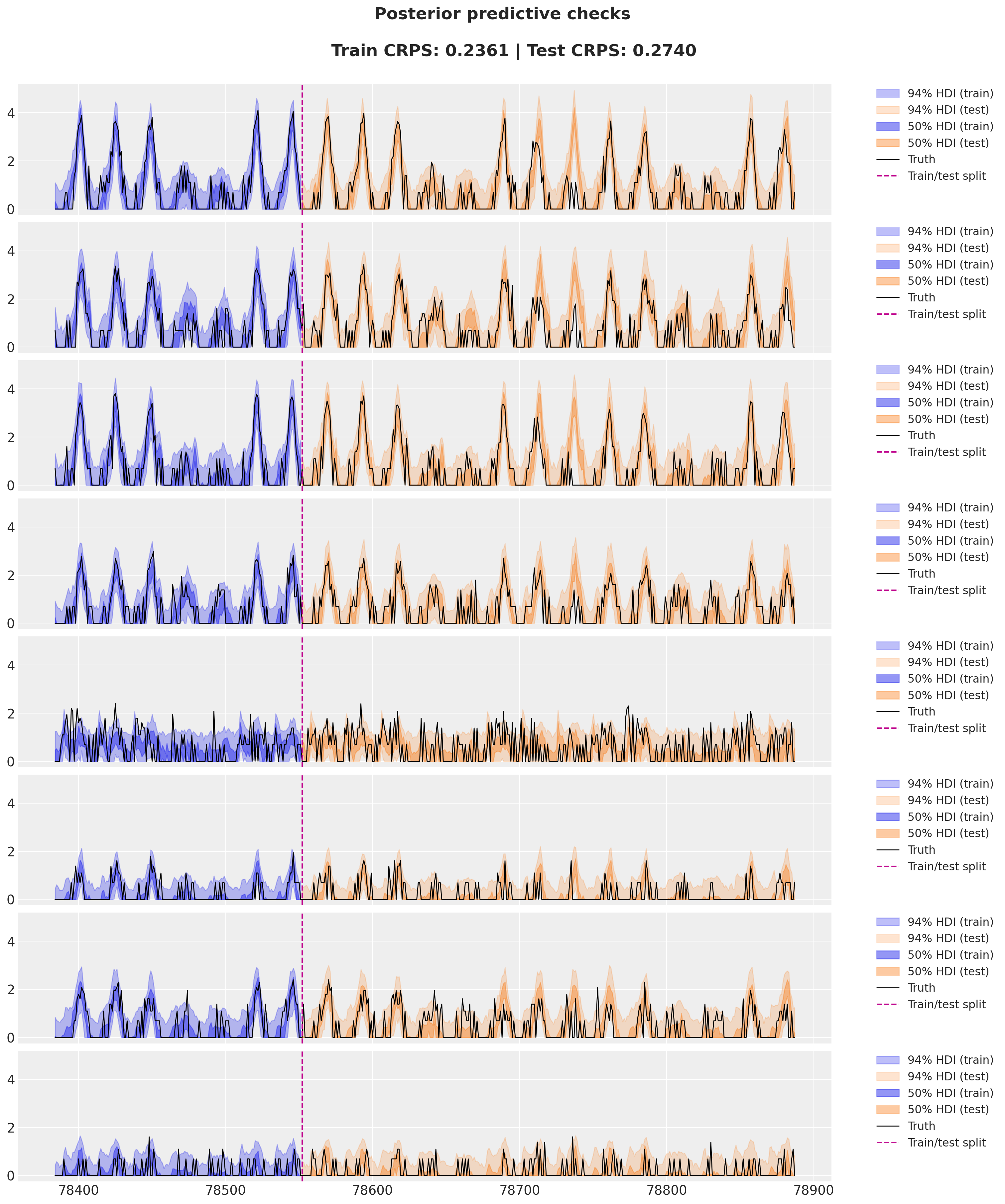
• End-to-End Example: Bayesian Neural Network Model

• Tips & Tricks

• References

Code

https://juanitorduz.github.io/intro_svi/

Demand Forecasting

Cohort Modeling

What is Variational Inference?

Bayes’ Rule

Recall, given the data \(D\) and the model \(p(\theta|D)\), we can use Bayes’ rule to compute the posterior distribution:

\[ p(\theta|D) = \frac{p(D|\theta)p(\theta)}{p(D)} \]

where:

• \(p(D|\theta)\): Likelihood (how well the model fits the data)
• \(p(\theta)\): Prior (our beliefs about the parameters before seeing the data)
• \(\displaystyle {p(D) = \int p(D|\theta)p(\theta)d\theta}\): Hard to compute!

• Stochastic Variational Inference (SVI) is a scalable approximate inference method that transforms the problem of posterior inference into an optimization problem.

• Instead of sampling from the posterior distribution (like MCMC), SVI finds the best approximation to the posterior within a family of simpler distributions.

Variational Inference in PyMC

JAX Ecosystem

JAX is a Python library for accelerator-oriented array computation and program transformation, designed for high-performance numerical computing and large-scale machine learning.

JAX

NumPyro

Flax

Optax

Variational Inference in a Nutshell

• \(D = \{(x_i, y_i)\}_{i=1}^N\): Our complete dataset

• \(\theta\): Model parameters (e.g., in a neural network, the weights and biases)

• \(p(\theta|D)\): True posterior distribution (what we want but can’t compute easily)

• \(q_\phi(\theta)\): Variational approximation to the posterior (what we’ll optimize)

• \(\phi\): Variational parameters (parameters of our approximate posterior)

---

• \(\text{ELBO}(\phi) = \mathbb{E}_{q_\phi(\theta)}[\log p(y|x, \theta)] - \text{KL}(q_\phi(\theta) || p(\theta))\)

• Maximizing the ELBO is equivalent to minimizing the KL divergence between our approximate posterior \(q_\phi(\theta)\) and the true posterior \(p(\theta|D)\) (up to a constant, with respect to \(q_\phi(\theta)\)). Why? Use the Bayes’ rule to expand the KL divergence.

• This decomposes into two intuitive terms:

  • \(\mathbb{E}_{q_\phi(\theta)}[\log p(y|x, \theta)]\): Expected log-likelihood (how well we explain the data)

  • \(\text{KL}(q_\phi(\theta) || p(\theta))\): KL divergence between \(q_\phi(\theta)\) and the prior \(p(\theta)\).

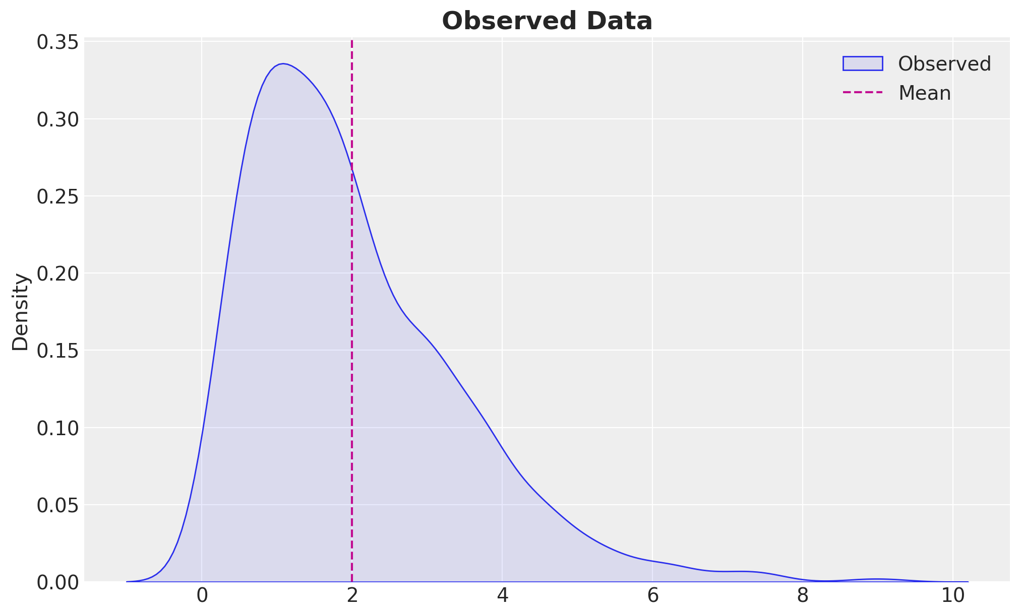
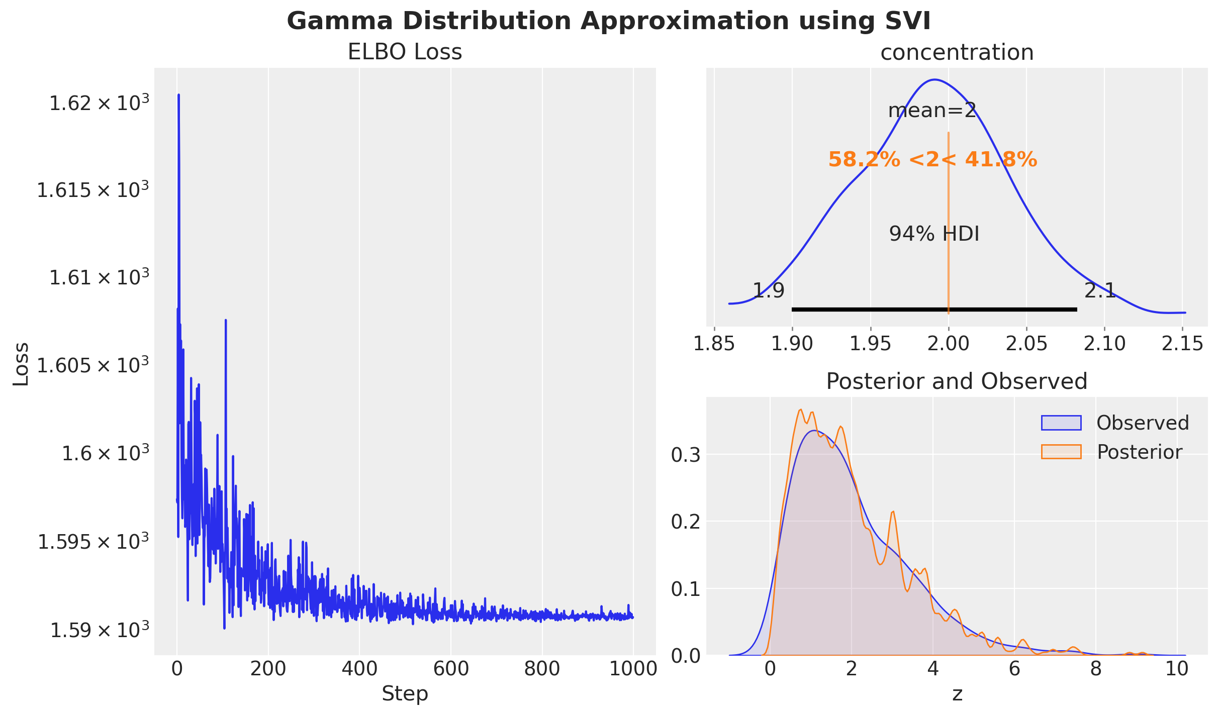
Estimating the Concentration Parameter of a Gamma Distribution \(\text{Gamma}(\alpha) \sim x^{\alpha - 1} e^{-x}\)

Approximation Model

We want to estimate the concentration parameter of a Gamma distribution. We model the data generating process as:

# Model to estimate the concentration parameter
def model(z: jax.Array | None = None) -> None:
    # Sample the concentration parameter from a HalfNormal distribution
    # as the concentration parameter has to be positive
    concentration = numpyro.sample(
        "concentration",
        dist.HalfNormal(scale=1),
    )
    # Sample the data from a Gamma distribution
    # with the concentration parameter and a rate of 1.0
    rate = 1.0
    numpyro.sample(
        "z",
        dist.Gamma(concentration=concentration, rate=rate),
        obs=z,
    )

Approximation Guide

def guide(z: jax.Array | None = None) -> None:
    # Location and scale parameters of the normal distribution
    concentration_loc = numpyro.param(
        "concentration_loc",
        init_value=0.5,
    )
    concentration_scale = numpyro.param(
        "concentration_scale",
        init_value=0.1,
        constraint=dist.constraints.positive,
    )
    # Variational approximation
    base_distribution = dist.Normal(
        loc=concentration_loc,
        scale=concentration_scale,
    )
    # We need to transform the base distribution
    # as the concentration parameter has to be positive
    transformed_distribution = dist.TransformedDistribution(
        base_distribution=base_distribution,
        transforms=dist.transforms.ExpTransform(),
    )
    # Sample the concentration parameter from the transformed distribution
    numpyro.sample("concentration", transformed_distribution)

Inference with SVI

This is how a typical SVI workflow looks like in NumPyro:

# Define the loss function (ELBO)
loss = Trace_ELBO(num_particles=10)

# Define the optimizer
optimizer = optax.adam(learning_rate=0.005)

# Define the SVI algorithm
svi = SVI(model=model, guide=guide, optim=optimizer, loss=loss)

# Run the SVI algorithm
rng_key, rng_subkey = random.split(rng_key)
svi_result = svi.run(
    rng_subkey,
    num_steps=1_000,
    z=z,
    progress_bar=True,
)

Approximation Results

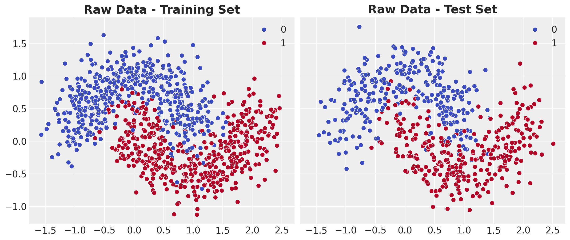
Example: Bayesian Neural Network

Classification problem with non-linear decision boundary.

Model Structure

Model Components

• We use a multi-layer perceptron (MLP) to model the non-linear decision boundary parameter \(p(x)\).
• We model our data with a Bernoulli likelihood with parameter \(p(x)\).

Neural Network Component 🤖

import jax
import jax.random as random
from flax import nnx
from itertools import pairwise


class MLP(nnx.Module):

    def __init__(
        self, din: int, dout: int, hidden_layers: list[int], *, rngs: nnx.Rngs
    ) -> None:
        self.layers = []

        layer_dims = [din, *hidden_layers, dout]

        for in_dim, out_dim in pairwise(layer_dims):
            self.layers.append(nnx.Linear(in_dim, out_dim, rngs=rngs))

    def __call__(self, x: jax.Array) -> jax.Array:
        for layer in self.layers[:-1]:
            x = jax.nn.tanh(layer(x))

        return jax.nn.sigmoid(self.layers[-1](x))


hidden_layers = [4, 3]
dout = 1
rng_key, rng_subkey = random.split(rng_key)
nnx_module = MLP(
    din=x_train.shape[1],
    dout=dout,
    hidden_layers=hidden_layers,
    rngs=nnx.Rngs(rng_subkey),
)

NumPyro Model

import numpyro
import numpyro.distributions as dist
from numpyro.contrib.module import random_nnx_module

def model(
    x: Float[Array, "n_obs features"],
    y: Int[Array, " n_obs"] | None = None,
) -> None:
    n_obs: int = x.shape[0]

    def prior(name, shape):
        if "bias" in name:
            return dist.Normal(loc=0, scale=1)
        return dist.SoftLaplace(loc=0, scale=1)

    nn = random_nnx_module(
        "nn",
        nnx_module,
        prior=prior,
    )

    p = numpyro.deterministic("p", nn(x).squeeze(-1))

    with numpyro.plate("data", n_obs):
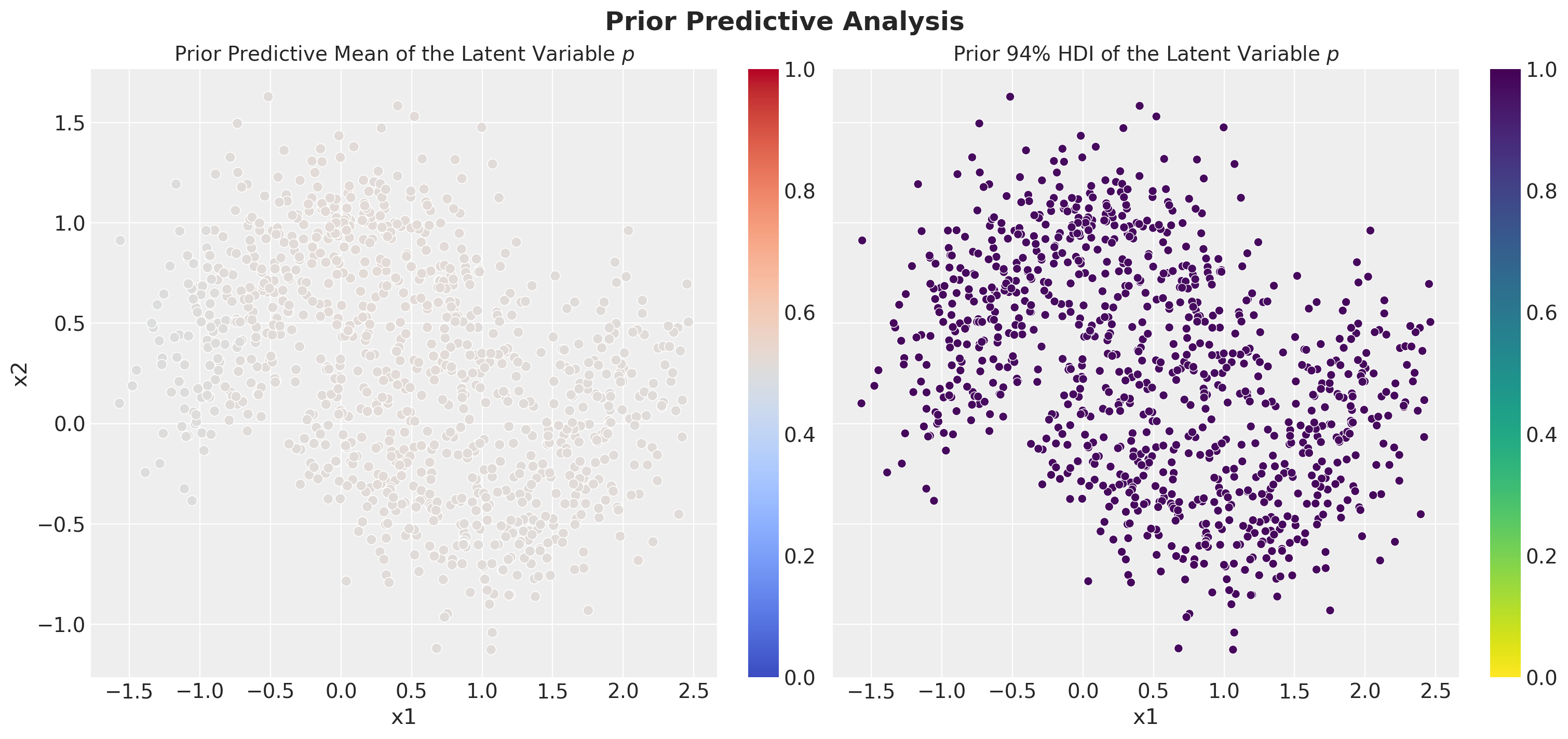
        numpyro.sample("y", dist.Bernoulli(probs=p), obs=y)

Prior Predictive Checks

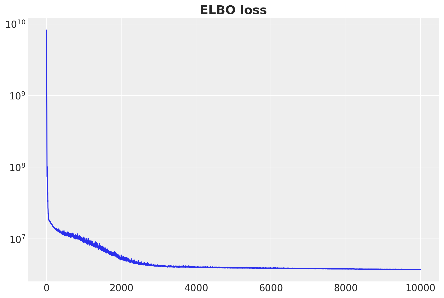
Inference: SVI in NumPyro 🚀

import numpyro
from numpyro.infer import SVI, Trace_ELBO
from numpyro.infer.autoguide import AutoNormal

guide = AutoNormal(model) # <- Posterior Approximation
optimizer = numpyro.optim.Adam(step_size=0.01) # <- Optimizer
svi = SVI(model, guide, optimizer, loss=Trace_ELBO())
num_steps = 10_000

rng_key, rng_subkey = random.split(key=rng_key)

# Optimization Loop
svi_result = svi.run(
    rng_subkey,
    num_steps,
    x_train,
    y_train,
)

# Results
params = svi_result.params

Inference: ELBO Curve

Inference: Custom Guide 🤕

def layer_guide(
    loc_shape: tuple[int, ...],
    loc_amplitude: float,
    scale_shape: tuple[int, ...],
    scale_amplitude: float,
    loc_name: str,
    scale_name: str,
    layer_name: str,
    event_shape: int = 1,
    seed: int = 42,
) -> None:

Writing a custom guide?

• If you are having trouble constructing a custom guide, use an AutoGuide.
• Parameter initialization matters: initialize guide distributions to have low variance.
• Pay attention to scales.

Inference: Custom Optimizer ⚡

import optax
# OneCycle schedule: low -> high -> low with specific timing
scheduler = optax.linear_onecycle_schedule(
    transition_steps=8_000,  # Total number of optimization steps
    peak_value=0.008,  # Maximum learning rate (reached at pct_start)
    pct_start=0.2,  # Percent of training to reach peak (20%)
    pct_final=0.8,  # Percent of training for final phase (80%)
    div_factor=3,  # Initial LR = peak_value / div_factor
    final_div_factor=4,  # Final LR = initial_LR / final_div_factor
)
# Chain multiple optimizers for sophisticated training
optimizer = optax.chain(
    # Primary optimizer: Adam with scheduled learning rate
    optax.adam(learning_rate=scheduler),
    # Secondary optimizer: Reduce LR when loss plateaus
    optax.contrib.reduce_on_plateau(
        factor=0.1,  # Multiply LR by 0.1 when plateau detected
        patience=10,  # Wait 10 evaluations before reducing
        accumulation_size=100,  # Window size for detecting plateaus
    ),
)

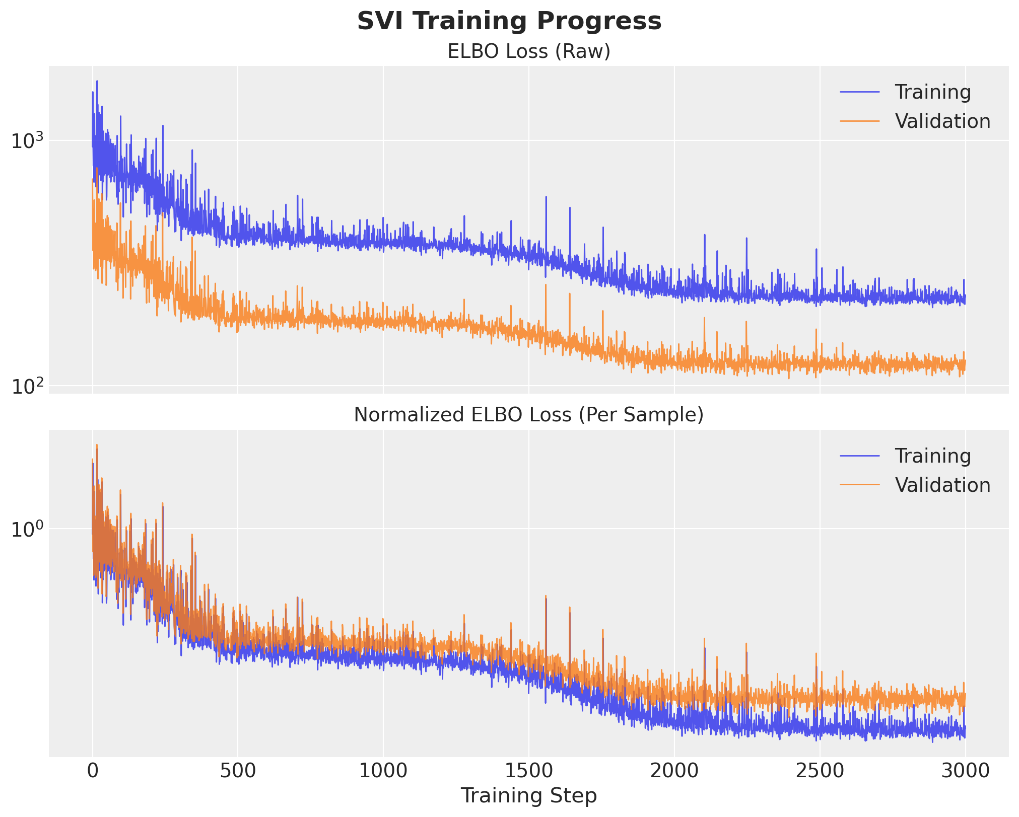
Inference: Custom Optimization Loop

def body_fn(svi_state, _):
    svi_state, loss = svi.update(svi_state, x=x_train, y=y_train)
    return svi_state, loss

with tqdm.trange(1, num_steps + 1) as t:
    batch = max(num_steps // 20, 1)
    patience_counter = 0

    for i in t:
        # Perform one training step (JIT compiled for speed)
        svi_state, train_loss = jax.jit(body_fn)(svi_state, None)

        # Normalize loss by dataset size for fair comparison
        norm_train_loss = jax.device_get(train_loss) / y_train.shape[0]
        train_losses.append(jax.device_get(train_loss))
        norm_train_losses.append(norm_train_loss)

        # Compute validation loss (JIT compiled for speed)
        val_loss = jax.jit(get_val_loss)(svi_state, x_val, y_val)
        norm_val_loss = jax.device_get(val_loss) / y_val.shape[0]
        val_losses.append(jax.device_get(val_loss))
        norm_val_losses.append(norm_val_loss)

        # Early stopping logic: stop if validation loss > training loss consistently
        condition = norm_val_loss > norm_train_loss
        patience_counter = patience_counter + 1 if condition else 0

        if patience_counter >= patience:
            print(
                f"Early stopping at step {i} (validation loss exceeding training loss)"
            )
            break

Inference: Early Stopping

37%|███▋      | 2924/8000 [00:02<00:04, 1145.56it/s, train: 396.8835, val: 202.2204]
Early stopping at step 2925 (validation loss exceeding training loss)

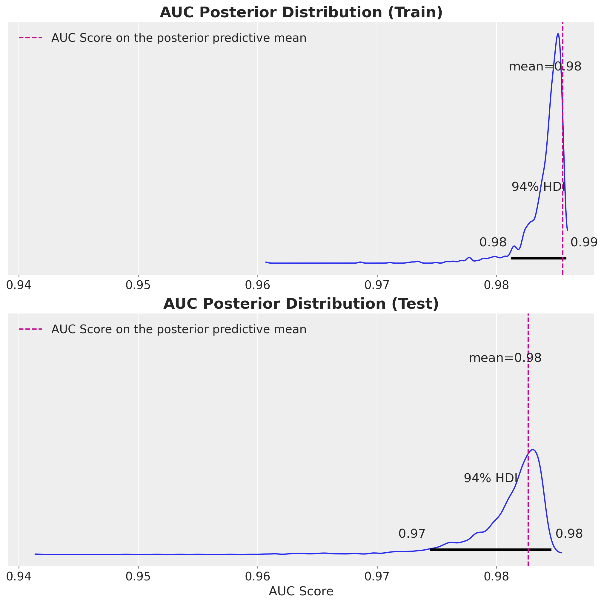
Model Evaluation: Posterior AUC

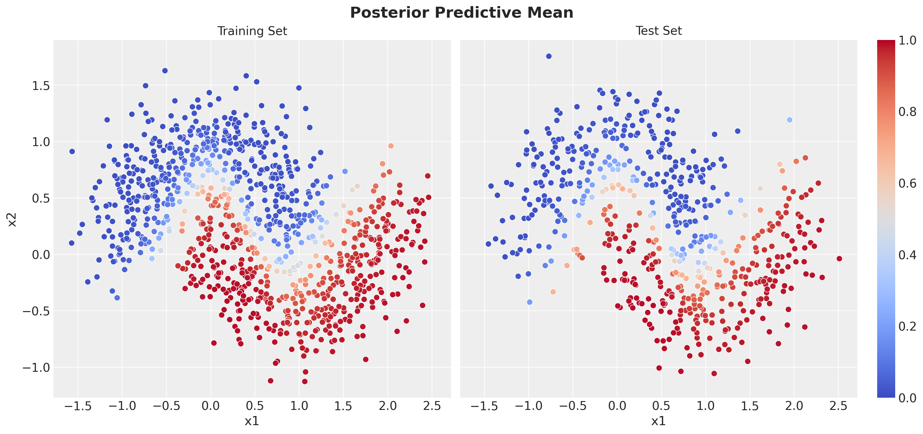
Posterior Predictive Mean

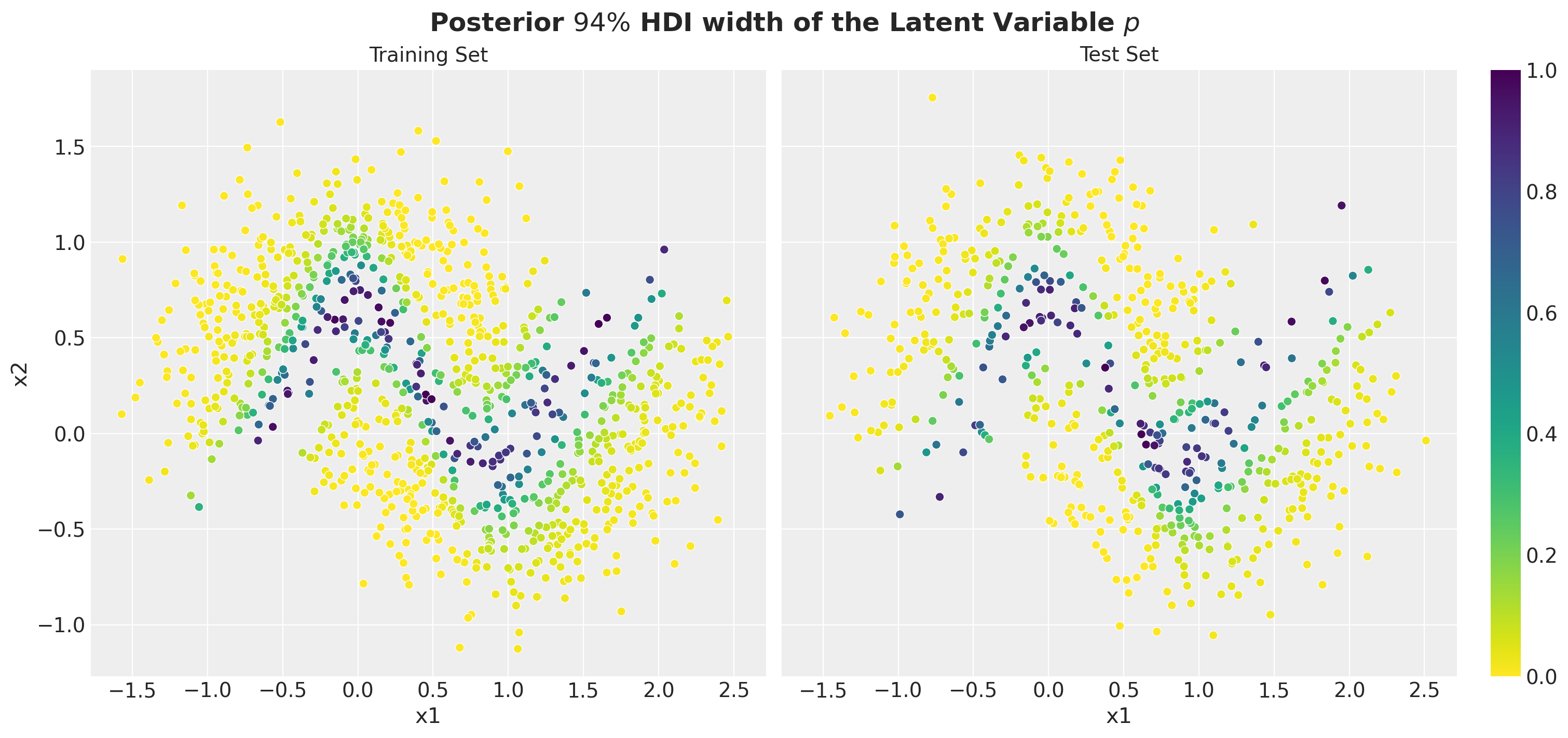
Posterior Predictive Uncertainty

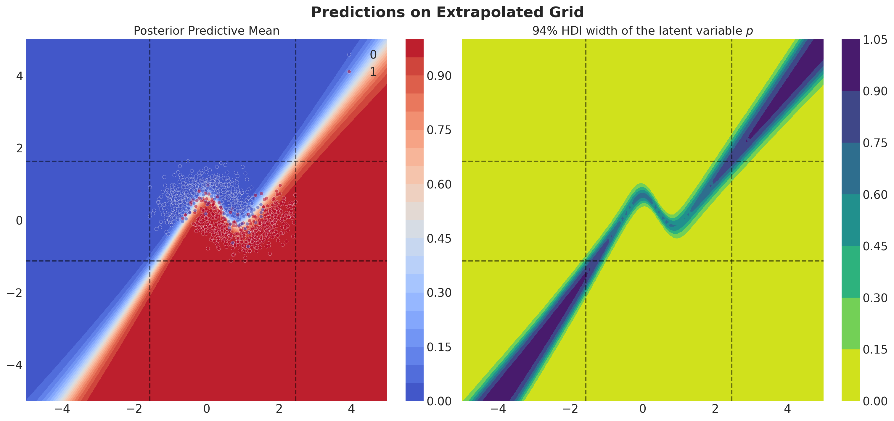
Predictions Outside Training Data

Tips & Tricks

When to Use SVI vs MCMC?

Use SVI when:

• You have large datasets
• You need fast inference for production systems
• You can accept approximate (vs exact) posterior inference

Use MCMC when:

• You have small-medium datasets
• You need precise posterior samples
• You have time for longer computation

Tips & Tricks

Tips and Tricks: SVI in Production

• Using GPUs for training can significantly speed up the training process.
• Using mini-batches can help with memory issues and speed up the training process.
• Using a good learning rate scheduler can help with the training process.
• Computing posterior predictive samples can be batched using Predictive from NumPyro (you might need to do it by hand, but is quite straightforward). This batching can help memory issues.

Other Inference Methods for Bayesian Models

It is important to note that there are other inference methods for Bayesian models:

• See all the Markov Chain Monte Carlo (MCMC) methods available in NumPyro
• See some more custom ones from Blackjax or FlowJAX.
• All of them can be integrated with NumPyro, see the example notebook NumPyro Integration with Other Libraries.

References 📚

Pyro Tutorials

• SVI Part I: An Introduction to Stochastic Variational Inference in Pyro
• SVI Part II: Conditional Independence, Subsampling, and Amortization
• SVI Part III: ELBO Gradient Estimators
• SVI Part IV: Tips and Tricks
• NumPyro Documentation

Papers

• Variational Inference: A Review for Statisticians
• Automatic Variational Inference in Stan

Videos

• Chris Fonnesbeck - A Beginner’s Guide to Variational Inference | PyData Virginia 2025

Thank you!

juanitorduz.github.io