In this notebook I want to experiment with some basic models for price elasticity estimation in the simple context of a simple sku across multiple stores and regions. The motivation is to have a concrete example of the elasticity models presented in the Chapter 11: Big Data Pricing Models of the book Pricing Analytics by Walter R. Paczkowski.
Elasticity Definition
Here I provide a very succinct definition of elasticity (there is a vast literature on this topic, see the reference above). The elasticity of a variable \(y(x, z)\) with respect to another variable \(x\) is defined as the percentage change in \(y\) for a one percent change in \(x\). Mathematically, this is written as \[ \eta = \frac{\partial \log(y(x, z))}{\partial \log(x)} \]
Example (log-log model): For example, if \(y(x) = ax^{b}\), then \(\log(y(x)) = \log(a) + b\log(x)\), which therefore implies \(\eta = b\) (this is referred as a log-log model). In this specific example the elasticity is constant.
Example (linear model): Now let us assume a linear relation \(y = a + bx\). Hence, from the chain rule, we have
\[ \eta = \frac{\partial \log(y(x))}{\partial \log(x)} = \frac{1}{y(x)}\frac{\partial y(x)}{\partial \log(x)} = \frac{1}{y(x)}x\frac{\partial y(x)}{\partial x} = \frac{xb}{y(x)} \]
Part 1: Data Generating Process
In this first part we study the data generating process in detail. This is important because it helps us understand the explicit assumptions we are making about the data and therefore how to build a model that is consistent with these assumptions.
Business Setting: We have a single sku across many stores across multiple regions. Each store has limited historical data regarding price and demand change over time. We want to estimate the price elasticity of demand for this sku in each store. We expect these elasticities differ across regions because of inherent differences in consumer income.
Prepare Notebook
import arviz as az
import matplotlib.pyplot as plt
import numpy as np
import pandas as pd
import pymc as pm
import pytensor.tensor as pt
import seaborn as sns

from numpy.typing import NDArray
from pydantic import BaseModel, Field, model_validator, field_validator
from tqdm.notebook import tqdm

az.style.use("arviz-darkgrid")
plt.rcParams["figure.figsize"] = [12, 7]
plt.rcParams["figure.dpi"] = 100
plt.rcParams["figure.facecolor"] = "white"

%load_ext autoreload
%autoreload 2
%config InlineBackend.figure_format = "retina"
seed: int = sum(map(ord, "multilevel_elasticities_single_sku"))
rng: np.random.Generator = np.random.default_rng(seed=seed)Entities Definition
The main objective of this first part is to generate data for each store. We want to generate price and demand data which reflects the heterogeneity of the regions, which have different media income which should have a considerable impact in consumer behavior.
Let us use pydantic to define the entities of our model. We will define the following entities:
class Sku(BaseModel):
    id: int = Field(..., ge=0)
    prices: NDArray[np.float_]
    quantities: NDArray[np.float_]

    class Config:
        arbitrary_types_allowed = True

    @field_validator("prices", "quantities")
    def validate_gt_0(cls, value):
        if (value <= 0).any():
            raise ValueError("prices and quantities must be positive")
        return value

    @field_validator("prices", "quantities")
    def validate_size_gt_0(cls, value):
        if value.size == 0:
            raise ValueError("prices and quantities must have at least one element")
        return value

    @model_validator(mode="before")
    def validate_sizes(cls, values):
        if values["prices"].size != values["quantities"].size:
            raise ValueError("prices and quantities must have the same size")
        return values

    def to_dataframe(self) -> pd.DataFrame:
        return pd.DataFrame(
            data={
                "item_id": self.id,
                "price": self.prices,
                "quantities": self.quantities,
                "time_step": np.arange(self.prices.size)[::-1],
            }
        )


class Store(BaseModel):
    id: int = Field(..., ge=0)
    items: list[Sku] = Field(..., min_items=1)

    @field_validator("items")
    def validate_item_ids(cls, value):
        if len({item.id for item in value}) != len(value):
            raise ValueError("items must have unique ids")
        return value

    def to_dataframe(self) -> pd.DataFrame:
        df = pd.concat([item.to_dataframe() for item in self.items], axis=0)
        df["store_id"] = self.id
        df["region_store_id"] = f"r-{self.id}_s-" + df["store_id"].astype(str)
        return df.reset_index(drop=True)


class Region(BaseModel):
    id: int = Field(..., ge=0)
    stores: list[Store] = Field(..., min_items=1)
    median_income: float = Field(..., gt=0)

    @field_validator("stores")
    def validate_store_ids(cls, value):
        if len({store.id for store in value}) != len(value):
            raise ValueError("stores must have unique ids")
        return value

    def to_dataframe(self) -> pd.DataFrame:
        df = pd.concat([store.to_dataframe() for store in self.stores], axis=0)
        df["region_id"] = self.id
        df["median_income"] = self.median_income
        return df.reset_index(drop=True)


class Market(BaseModel):
    regions: list[Region] = Field(..., min_items=1)

    @field_validator("regions")
    def validate_region_ids(cls, value):
        if len({region.id for region in value}) != len(value):
            raise ValueError("regions must have unique ids")
        return value

    def to_dataframe(self) -> pd.DataFrame:
        df = pd.concat([region.to_dataframe() for region in self.regions], axis=0)
        return df.reset_index(drop=True).assign(
            log_price=lambda x: np.log(x["price"]),
            log_quantities=lambda x: np.log(x["quantities"]),
            region_id=lambda x: x["region_id"].astype("category"),
            region_store_id=lambda x: x["region_store_id"].astype("category"),
        )
Model Specification
We are going to focus on the varying-intercept and varying intercept-slope model. Let us denote our target variable of interest by \(y\) (e.g. log quantity) and our treatment variable by \(x\) (e.g. log prices). By varying-intercept/slope we mean that the intercept and slope of the linear model to model \(y\) with \(x\) vary stochastically as a function of some regional-dependent variables (e.g. mean income). Concretely, then the varying-intercept model is given by
\[\begin{align*} y_{it} &= \alpha_{j[i]} + \beta_{j[i]} x_{it} + \varepsilon_{i} \\ \alpha_{j} &= \alpha^{\text{intercept}} + \alpha^{\text{slope}} z_{j} + \gamma_{0j} \\ \beta_{j} &= \beta^{\text{intercept}} + \beta^{\text{slope}} w_{j} + \gamma_{1j} \end{align*}\]
where \(j = 1, \cdots, J\) denote the regions, \(j[i]\) is region associated to the store \(i\), \(z_{j}, w_{j}\) are features of each region and \(\varepsilon\), \(\gamma_{0j}\) and \(\gamma_{1j}\) denote Gaussian noise. We are mainly interested in \(\beta_{j[i]}\) to estimate the elasticities of the demand (see examples above). For more information and a complete comparison of related model pease refer to Chapter 11: Big Data Pricing Models of the book Pricing Analytics by Walter R. Paczkowski, the main reference of this notebook.
Data Generating Process
We are going to generate data from a log-log price demand model. In order to make the mathematical model more tangible, it is very instructive to code it explicitly 🤓. To start, please note we need to encode linear regression parameters. This motivates to define the following data model:
class LinearRegressionConfig(BaseModel):
    intercept: float
    slope: float
    sigma: float = Field(..., gt=0)
Now we develop the core implementation of the data generating process. One thing to notice is that we are not pre-define the number of stores per region or the store-specific price history. We are going to randomly sample from negative binomial distributions (note we are going to use seeds to make everything fully reproducible). Similarly, we get the median income per region as sames from a gamma distribution.
The following class encapsulates the atomic steps of the data generating process as methods. The explicit methods and parameter names and code structure should (hopefully!) make the code self-explanatory.
class MultiLevelElasticitiesDataGenerator(BaseModel):
    rng: np.random.Generator
    n_regions: int = Field(..., gt=0)
    time_range_mu: float = Field(..., gt=0)
    time_range_sigma: float = Field(..., gt=0)
    n_stores_per_region_mu: float = Field(..., gt=0)
    n_stores_per_region_sigma: float = Field(..., gt=0)
    median_income_per_region_mu: float = Field(..., gt=0)
    median_income_per_region_sigma: float = Field(..., gt=0)
    intercepts_lr_config: LinearRegressionConfig
    slopes_lr_config: LinearRegressionConfig
    price_mu: float = Field(..., gt=0)
    price_sigma: float = Field(..., gt=0)
    epsilon: float = Field(..., gt=0)

    class Config:
        arbitrary_types_allowed = True

    def get_n_stores_per_region_draws(self) -> NDArray:
        n_stores_per_region_dist = pm.NegativeBinomial.dist(
            mu=self.n_stores_per_region_mu, alpha=self.n_stores_per_region_sigma
        )
        n_stores_per_region_draws = pm.draw(
            n_stores_per_region_dist, draws=self.n_regions, random_seed=self.rng
        )
        return n_stores_per_region_draws + 2

    def get_median_income_per_region_draws(self) -> NDArray:
        median_income_per_region_dist = pm.Gamma.dist(
            mu=self.median_income_per_region_mu,
            sigma=self.median_income_per_region_sigma,
        )
        median_income_per_region_draws = pm.draw(
            median_income_per_region_dist, draws=self.n_regions, random_seed=self.rng
        )
        return median_income_per_region_draws + 1

    def get_store_time_range(self) -> int:
        time_range_dist = pm.NegativeBinomial.dist(
            mu=self.time_range_mu, alpha=self.time_range_sigma
        )
        time_range_samples = pm.draw(
            vars=time_range_dist, draws=1, random_seed=self.rng
        ).item()
        return time_range_samples + 2

    def get_alpha_j_samples(
        self, median_income_per_region: float, store_time_range: int
    ) -> NDArray:
        alpha_j_dist = pm.Normal.dist(
            mu=self.intercepts_lr_config.intercept
            + self.intercepts_lr_config.slope * median_income_per_region,
            sigma=self.intercepts_lr_config.sigma,
        )
        return pm.draw(alpha_j_dist, draws=store_time_range, random_seed=self.rng)

    def get_beta_j_samples(
        self, median_income_per_region: float, store_time_range: int
    ) -> NDArray:
        beta_j_dist = pm.Normal.dist(
            mu=self.slopes_lr_config.intercept
            + self.slopes_lr_config.slope * median_income_per_region,
            sigma=self.slopes_lr_config.sigma,
        )
        return pm.draw(beta_j_dist, draws=store_time_range, random_seed=self.rng)

    def get_prices_samples(self, store_time_range: int) -> NDArray:
        price_dist = pm.Gamma.dist(
            mu=self.price_mu,
            sigma=self.price_sigma,
        )
        return pm.draw(price_dist, draws=store_time_range, random_seed=self.rng)

    def get_quantities_samples(
        self, alpha_j_samples, beta_j_samples, prices_samples
    ) -> NDArray:
        log_quantities_dist = pm.Normal.dist(
            mu=alpha_j_samples + beta_j_samples * np.log(prices_samples),
            sigma=self.epsilon,
        )
        log_quantities_samples = pm.draw(
            log_quantities_dist, draws=1, random_seed=self.rng
        )
        return np.exp(log_quantities_samples)

    def create_store(self, id: int, median_income_per_region: float) -> Store:
        store_time_range = self.get_store_time_range()
        alpha_j_samples = self.get_alpha_j_samples(
            median_income_per_region=median_income_per_region,
            store_time_range=store_time_range,
        )
        beta_j_samples = self.get_beta_j_samples(
            median_income_per_region=median_income_per_region,
            store_time_range=store_time_range,
        )
        prices_samples = self.get_prices_samples(store_time_range=store_time_range)
        quantities_samples = self.get_quantities_samples(
            alpha_j_samples=alpha_j_samples,
            beta_j_samples=beta_j_samples,
            prices_samples=prices_samples,
        )
        return Store(
            id=id,
            items=[
                Sku(id=0, prices=prices_samples, quantities=quantities_samples)
            ],  # <- we only have one sku (id = 0)
        )

    def create_region(
        self, id: int, n_stores_per_region: int, median_income_per_region: float
    ) -> Region:
        stores: list[Store] = [
            self.create_store(id=i, median_income_per_region=median_income_per_region)
            for i in range(n_stores_per_region)
        ]
        return Region(id=id, stores=stores, median_income=median_income_per_region)

    def run(self) -> Market:
        n_stores_per_region_draws = self.get_n_stores_per_region_draws()
        median_income_per_region_draws = self.get_median_income_per_region_draws()

        regions: list[Region] = [
            self.create_region(
                id=j,
                n_stores_per_region=n_stores_per_region_draws[j],
                median_income_per_region=median_income_per_region_draws[j],
            )
            for j in tqdm(range(self.n_regions))
        ]

        return Market(regions=regions)
Remark: The quantities field is a float number which can be interpreted as units of a thousand. For example, the value 1.5 means 1,500 units.
We now specify explicit input parameters to generate a market.
data_generator = MultiLevelElasticitiesDataGenerator(
    rng=rng,
    n_regions=9,
    time_range_mu=20,
    time_range_sigma=5,
    n_stores_per_region_mu=10,
    n_stores_per_region_sigma=3,
    median_income_per_region_mu=5,
    median_income_per_region_sigma=2,
    intercepts_lr_config=LinearRegressionConfig(intercept=1, slope=0.3, sigma=0.02),
    slopes_lr_config=LinearRegressionConfig(intercept=-0.1, slope=-0.6, sigma=0.02),
    price_mu=1.5,
    price_sigma=0.25,
    epsilon=0.3,
)
We finally get our data!
market = data_generator.run()

market_df = market.to_dataframe()

market_df.head()| item_id | price | quantities | time_step | store_id | region_store_id | region_id | median_income | log_price | log_quantities | |
|---|---|---|---|---|---|---|---|---|---|---|
| 0 | 0 | 1.335446 | 6.170862 | 16 | 0 | r-0_s-0 | 0 | 5.873343 | 0.289265 | 1.819839 |
| 1 | 0 | 1.702792 | 3.715124 | 15 | 0 | r-0_s-0 | 0 | 5.873343 | 0.532269 | 1.312412 |
| 2 | 0 | 1.699778 | 3.290962 | 14 | 0 | r-0_s-0 | 0 | 5.873343 | 0.530498 | 1.191180 |
| 3 | 0 | 1.335844 | 5.702928 | 13 | 0 | r-0_s-0 | 0 | 5.873343 | 0.289563 | 1.740980 |
| 4 | 0 | 1.517213 | 4.264949 | 12 | 0 | r-0_s-0 | 0 | 5.873343 | 0.416875 | 1.450430 |
EDA
Before any modeling, it is important to do a proper explanatory data analysis!
First, we visualize samples of the store prices and quantities for a selected region:
fig, ax = plt.subplots(
    nrows=2, ncols=1, figsize=(12, 8), sharex=True, sharey=False, layout="constrained"
)

region = 3

sns.lineplot(
    data=market_df.query("region_id == @region").assign(
        store_id=lambda x: x["store_id"].astype("category")
    ),
    x="time_step",
    y="price",
    hue="store_id",
    marker="o",
    ax=ax[0],
)
ax[0].invert_xaxis()
ax[0].legend(
    title="Store ID", title_fontsize=14, loc="center left", bbox_to_anchor=(1, 0.5)
)
ax[0].set(xlabel="Time Step", ylabel="Price")
ax[0].set_title(
    label=f"Prices by Store in Region {region}", fontsize=18, fontweight="bold"
)

sns.lineplot(
    data=market_df.query("region_id == 3").assign(
        store_id=lambda x: x["store_id"].astype("category")
    ),
    x="time_step",
    y="quantities",
    hue="store_id",
    marker="o",
    ax=ax[1],
)
ax[1].legend(
    title="Store ID", title_fontsize=14, loc="center left", bbox_to_anchor=(1, 0.5)
)
ax[1].set(xlabel="Time Step", ylabel="Quantity")
ax[1].set_title(
    label=f"Quantities by Store in Region {region}", fontsize=18, fontweight="bold"
)
Note that The Sore \(0\) has \(9\) data points of historical prices. Estimating the elasticity for the SKU with a regression at a store level would be very noisy. This motivates the use of a multilevel model through the regions.
Next, we plot the demand as a function of price for each region.
g = sns.relplot(
    data=market_df,
    x="price",
    y="quantities",
    kind="scatter",
    col="region_id",
    col_wrap=3,
    hue="region_id",
    height=3.5,
    aspect=1,
    facet_kws={"sharex": True, "sharey": True},
)
legend = g.legend
legend.set_title(title="Region ID", prop={"size": 10})
g.fig.suptitle(
    "Prices vs Quantities by Region", y=1.05, fontsize=18, fontweight="bold"
)

We do see heterogeneity in the elasticities across the different regions. Let’s look this data into a log-log scale:
g = sns.lmplot(
    data=market_df,
    x="log_price",
    y="log_quantities",
    hue="region_id",
    height=8,
    aspect=1.2,
    scatter=False,
)
g.set_axis_labels(x_var="Log Prices", y_var="Log Quantities")
legend = g.legend
legend.set_title(title="Region ID", prop={"size": 10})
g.fig.suptitle(
    "Log Prices vs Log Quantities by Region", y=1.05, fontsize=18, fontweight="bold"
)

From our data generating process, we expect the slopes and intercepts to be related to the mean_income feature per region.
fig, ax = plt.subplots(figsize=(9, 6))
(
    market_df.groupby("region_id", as_index=False)
    .agg({"median_income": np.mean})
    .pipe((sns.barplot, "data"), x="region_id", y="median_income", ax=ax)
)
ax.set(xlabel="Region ID", ylabel="Median Income")
ax.set_title(label="Median Income by Region", fontsize=18, fontweight="bold")
Part 2: Multilevel Elasticities Model
In this second part we focus on the elasticity models. As always, we start with a simple baseline model and then add more complexity.
Baseline Model
As a baseline we model each region independently, with no interaction between regions. We expect high variance for the estimates of the elasticities, specially for region \(3\) since it only has two stores.
We star by formatting the data used in the models.
obs = market_df.index.to_numpy()
price = market_df["price"].to_numpy()
log_price = market_df["log_price"].to_numpy()
quantities = market_df["quantities"].to_numpy()
log_quantities = market_df["log_quantities"].to_numpy()
median_income_idx, median_income = market_df["median_income"].factorize(sort=True)
region_idx, region = market_df["region_id"].factorize(sort=True)
Next, we specify the base model.
coords = {"region": region, "obs": obs}

with pm.Model(coords=coords) as base_model:
    # --- Priors ---
    alpha_j = pm.Normal(name="alpha_j", mu=0, sigma=1.5, dims="region")
    beta_j = pm.Normal(name="beta_j", mu=0, sigma=1.5, dims="region")
    sigma = pm.Exponential(name="sigma", lam=1 / 0.5)
    # --- Parametrization ---
    alpha = pm.Deterministic(name="alpha", var=alpha_j[region_idx], dims="obs")
    beta = pm.Deterministic(name="beta", var=beta_j[region_idx], dims="obs")
    mu = pm.Deterministic(name="mu", var=alpha + beta * log_price, dims="obs")
    # --- Likelihood ---
    pm.Normal(
        name="likelihood", mu=mu, sigma=sigma, observed=log_quantities, dims="obs"
    )

pm.model_to_graphviz(model=base_model)
Before fitting the model, we sample from the model to asses the prior predictive distribution. This is a good way to check that the model is well specified. We can also use this to check that the model is able to generate data that is similar to the observed data.
with base_model:
    prior_predictive_base = pm.sample_prior_predictive(samples=1_000, random_seed=rng)
fig, ax = plt.subplots(figsize=(12, 7))
az.plot_ppc(data=prior_predictive_base, group="prior", kind="kde", ax=ax)
ax.set_title(label="Base Model - Prior Predictive", fontsize=18, fontweight="bold")

The prior-predictive samples look very reasonable. Now we proceed to fit the model.
with base_model:
    idata_base = pm.sample(
        target_accept=0.9,
        draws=6_000,
        chains=5,
        nuts_sampler="numpyro",
        random_seed=rng,
        idata_kwargs={"log_likelihood": True},
    )
    posterior_predictive_base = pm.sample_posterior_predictive(
        trace=idata_base, random_seed=rng
    )
Let’s see the estimated distributions and diagnostics.
# number of divergences
idata_base["sample_stats"]["diverging"].sum().item()
0var_names = [
"alpha_j",
"beta_j",
"sigma",
]
az.summary(data=idata_base, var_names=var_names, round_to=2)| mean | sd | hdi_3% | hdi_97% | mcse_mean | mcse_sd | ess_bulk | ess_tail | r_hat | |
|---|---|---|---|---|---|---|---|---|---|
| alpha_j[0] | 2.75 | 0.05 | 2.65 | 2.84 | 0.0 | 0.0 | 37375.99 | 22008.01 | 1.0 |
| alpha_j[1] | 2.98 | 0.06 | 2.88 | 3.09 | 0.0 | 0.0 | 39085.34 | 20307.70 | 1.0 |
| alpha_j[2] | 2.44 | 0.03 | 2.38 | 2.51 | 0.0 | 0.0 | 38652.57 | 21388.95 | 1.0 |
| alpha_j[3] | 3.50 | 0.13 | 3.26 | 3.74 | 0.0 | 0.0 | 37371.38 | 21246.46 | 1.0 |
| alpha_j[4] | 2.97 | 0.05 | 2.87 | 3.06 | 0.0 | 0.0 | 35995.13 | 20938.54 | 1.0 |
| alpha_j[5] | 2.83 | 0.06 | 2.71 | 2.93 | 0.0 | 0.0 | 41063.64 | 21439.40 | 1.0 |
| alpha_j[6] | 3.07 | 0.05 | 2.98 | 3.16 | 0.0 | 0.0 | 38274.60 | 22013.66 | 1.0 |
| alpha_j[7] | 2.34 | 0.03 | 2.29 | 2.40 | 0.0 | 0.0 | 38568.20 | 20446.92 | 1.0 |
| alpha_j[8] | 2.53 | 0.04 | 2.46 | 2.60 | 0.0 | 0.0 | 40067.32 | 22195.92 | 1.0 |
| beta_j[0] | -3.54 | 0.12 | -3.76 | -3.32 | 0.0 | 0.0 | 37574.35 | 21532.12 | 1.0 |
| beta_j[1] | -4.06 | 0.13 | -4.30 | -3.81 | 0.0 | 0.0 | 40448.37 | 19859.76 | 1.0 |
| beta_j[2] | -2.98 | 0.08 | -3.14 | -2.83 | 0.0 | 0.0 | 38958.73 | 20303.17 | 1.0 |
| beta_j[3] | -5.10 | 0.32 | -5.68 | -4.49 | 0.0 | 0.0 | 37340.00 | 20279.28 | 1.0 |
| beta_j[4] | -3.96 | 0.12 | -4.19 | -3.73 | 0.0 | 0.0 | 36650.88 | 21317.61 | 1.0 |
| beta_j[5] | -3.59 | 0.13 | -3.85 | -3.34 | 0.0 | 0.0 | 40357.11 | 21684.55 | 1.0 |
| beta_j[6] | -4.16 | 0.11 | -4.37 | -3.95 | 0.0 | 0.0 | 38412.22 | 21625.78 | 1.0 |
| beta_j[7] | -2.79 | 0.07 | -2.91 | -2.66 | 0.0 | 0.0 | 37725.31 | 20520.08 | 1.0 |
| beta_j[8] | -3.20 | 0.09 | -3.37 | -3.03 | 0.0 | 0.0 | 40115.13 | 22093.00 | 1.0 |
| sigma | 0.29 | 0.00 | 0.28 | 0.30 | 0.0 | 0.0 | 49119.46 | 21077.52 | 1.0 |
As expected all the elasticities (\(\beta_{j}\)) are negative. Let’s look into the model trace to get a better glimpse of the posterior distribution of the parameters.
axes = az.plot_trace(
    data=idata_base,
    var_names=var_names,
    compact=True,
    backend_kwargs={"figsize": (12, 7), "layout": "constrained"},
)
plt.gcf().suptitle("Base Model - Trace", fontsize=18, fontweight="bold")

It is interesting to see that the variance of Region \(3\) is much higher than the variance the other stores. This is not surprising given the number of stores it has. We can zoom in to better compare the posterior distribution of the elasticities:
ax, *_ = az.plot_forest(
    data=idata_base,
    var_names=["beta_j"],
    combined=True,
    figsize=(8, 6),
)
ax.set_title(label="Base Model", fontsize=18, fontweight="bold")

We can also plot the estimated quantities posterior distribution (likelihood) as a function of price:
exp_likelihood_hdi = az.hdi(
    ary=np.exp(posterior_predictive_base["posterior_predictive"]["likelihood"])
)["likelihood"]

g = sns.relplot(
    data=market_df,
    x="price",
    y="quantities",
    kind="scatter",
    col="region_id",
    col_wrap=3,
    hue="region_id",
    height=3.5,
    aspect=1,
    facet_kws={"sharex": True, "sharey": True},
)

axes = g.axes.flatten()

for i, region_to_plot in enumerate(region):
    ax = axes[i]

    price_region = price[region_idx == region_to_plot]
    price_region_argsort = np.argsort(price_region)

    ax.fill_between(
        x=price_region[price_region_argsort],
        y1=exp_likelihood_hdi[region_idx == region_to_plot][price_region_argsort, 0],
        y2=exp_likelihood_hdi[region_idx == region_to_plot][price_region_argsort, 1],
        color=f"C{i}",
        alpha=0.2,
    )

legend = g.legend
legend.set_title(title="Region ID", prop={"size": 10})
g.fig.suptitle(
    "Prices vs Quantities by Region - Base Model",
    y=1.05,
    fontsize=18,
    fontweight="bold",
)

Note that Region \(3\) high variance a price \(1\$\) which is not present in other stores. As we are modeling the regions independently we do not expect the price elasticity information to be pooled across regions. Still, as it is the same product (same brand), we might expect a global effect of the price on the demand. This motivates the next models.
Multilevel Model
The next multilevel model mimics the data generating process of MultiLevelElasticitiesDataGenerator, so we expect it to recover the true parameters. We use a non-centered parameterization of the random effects, which is more efficient for sampling.
coords = {"region": region, "obs": obs}

with pm.Model(coords=coords) as model:
    # --- Priors ---
    alpha_j_intercept = pm.Normal(name="alpha_j_intercept", mu=0, sigma=0.5)
    alpha_j_slope = pm.Normal(name="alpha_j_slope", mu=0, sigma=0.3)
    sigma_alpha = pm.Exponential(name="sigma_alpha", lam=1 / 0.05)
    z_alpha_j = pm.Normal(name="z_alpha_j", mu=0, sigma=1, dims="region")

    beta_j_intercept = pm.Normal(name="beta_j_intercept", mu=0, sigma=0.5)
    beta_j_slope = pm.Normal(name="beta_j_slope", mu=0, sigma=0.3)
    sigma_beta = pm.Exponential(name="sigma_beta", lam=1 / 0.05)
    z_beta_j = pm.Normal(name="z_beta_j", mu=0, sigma=1, dims="region")

    sigma = pm.Exponential(name="sigma", lam=1 / 0.5)

    # --- Parametrization ---
    alpha_j_mu = pm.Deterministic(
        name="alpha_j_mu",
        var=alpha_j_intercept + alpha_j_slope * median_income.to_numpy(),
        dims="region",
    )
    alpha_j_sigma = pm.Deterministic(
        name="alpha_j_sigma", var=sigma_alpha * z_alpha_j, dims="region"
    )
    alpha_j = pm.Deterministic(
        name="alpha_j",
        var=alpha_j_mu + alpha_j_sigma,
        dims="region",
    )

    beta_j_mu = pm.Deterministic(
        name="beta_j_mu",
        var=beta_j_intercept + beta_j_slope * median_income.to_numpy(),
        dims="region",
    )
    beta_j_sigma = pm.Deterministic(
        name="beta_j_sigma", var=sigma_beta * z_beta_j, dims="region"
    )
    beta_j = pm.Deterministic(
        name="beta_j",
        var=beta_j_mu + beta_j_sigma,
        dims="region",
    )

    alpha = pm.Deterministic(name="alpha", var=alpha_j[region_idx], dims="obs")
    beta = pm.Deterministic(name="beta", var=beta_j[region_idx], dims="obs")

    mu = pm.Deterministic(name="mu", var=alpha + beta * log_price, dims="obs")

    # --- Likelihood ---
    pm.Normal(
        name="likelihood", mu=mu, sigma=sigma, observed=log_quantities, dims="obs"
    )

pm.model_to_graphviz(model=model)

We again start by looking into the prior predictive distribution of the model.
with model:
    prior_predictive = pm.sample_prior_predictive(samples=1_000, random_seed=rng)
fig, ax = plt.subplots(figsize=(12, 7))
az.plot_ppc(data=prior_predictive, group="prior", kind="kde", ax=ax)
ax.set_title(
label="Multilevel Model - Prior Predictive", fontsize=18, fontweight="bold"
)

We see our priors are not very informative. We now fit the model.
with model:
    idata = pm.sample(
        target_accept=0.9,
        draws=6_000,
        chains=5,
        nuts_sampler="numpyro",
        random_seed=rng,
        idata_kwargs={"log_likelihood": True},
    )
    posterior_predictive = pm.sample_posterior_predictive(
        trace=idata, random_seed=rng
    )
This model takes considerably longer to run than the previous one, but it is still feasible to run it on a laptop (\(6\) minutes in a Intel MacBook Pro). Next, we go through some diagnostics and the inferred parameters.
idata["sample_stats"]["diverging"].sum().item()0var_names = [
"alpha_j_intercept",
"alpha_j_slope",
"beta_j_intercept",
"beta_j_slope",
"alpha_j",
"beta_j",
"sigma",
]
az.summary(data=idata, var_names=var_names, round_to=2)| mean | sd | hdi_3% | hdi_97% | mcse_mean | mcse_sd | ess_bulk | ess_tail | r_hat | |
|---|---|---|---|---|---|---|---|---|---|
| alpha_j_intercept | 1.32 | 0.48 | 0.43 | 2.20 | 0.0 | 0.0 | 14978.93 | 15935.20 | 1.0 |
| alpha_j_slope | 0.23 | 0.08 | 0.08 | 0.36 | 0.0 | 0.0 | 15192.69 | 16569.44 | 1.0 |
| beta_j_intercept | -1.03 | 0.48 | -1.93 | -0.13 | 0.0 | 0.0 | 21221.32 | 18094.11 | 1.0 |
| beta_j_slope | -0.40 | 0.08 | -0.55 | -0.25 | 0.0 | 0.0 | 20596.83 | 18710.78 | 1.0 |
| alpha_j[0] | 2.74 | 0.05 | 2.65 | 2.83 | 0.0 | 0.0 | 37117.87 | 26498.29 | 1.0 |
| alpha_j[1] | 2.97 | 0.06 | 2.86 | 3.07 | 0.0 | 0.0 | 38832.36 | 26849.65 | 1.0 |
| alpha_j[2] | 2.45 | 0.03 | 2.38 | 2.51 | 0.0 | 0.0 | 33206.54 | 24310.89 | 1.0 |
| alpha_j[3] | 3.38 | 0.13 | 3.14 | 3.61 | 0.0 | 0.0 | 31832.99 | 21982.24 | 1.0 |
| alpha_j[4] | 2.97 | 0.05 | 2.87 | 3.06 | 0.0 | 0.0 | 40252.55 | 24868.84 | 1.0 |
| alpha_j[5] | 2.84 | 0.06 | 2.74 | 2.95 | 0.0 | 0.0 | 42852.82 | 23601.94 | 1.0 |
| alpha_j[6] | 3.07 | 0.05 | 2.98 | 3.16 | 0.0 | 0.0 | 37637.96 | 26125.46 | 1.0 |
| alpha_j[7] | 2.36 | 0.03 | 2.30 | 2.41 | 0.0 | 0.0 | 31100.91 | 25367.20 | 1.0 |
| alpha_j[8] | 2.56 | 0.04 | 2.49 | 2.63 | 0.0 | 0.0 | 32050.96 | 25922.67 | 1.0 |
| beta_j[0] | -3.53 | 0.12 | -3.75 | -3.31 | 0.0 | 0.0 | 37677.58 | 25205.56 | 1.0 |
| beta_j[1] | -4.02 | 0.13 | -4.25 | -3.78 | 0.0 | 0.0 | 39052.97 | 24705.54 | 1.0 |
| beta_j[2] | -3.00 | 0.08 | -3.15 | -2.85 | 0.0 | 0.0 | 33974.61 | 22489.06 | 1.0 |
| beta_j[3] | -4.79 | 0.31 | -5.37 | -4.22 | 0.0 | 0.0 | 32496.57 | 20896.10 | 1.0 |
| beta_j[4] | -3.96 | 0.12 | -4.18 | -3.74 | 0.0 | 0.0 | 40635.18 | 23390.98 | 1.0 |
| beta_j[5] | -3.63 | 0.13 | -3.88 | -3.38 | 0.0 | 0.0 | 43905.95 | 22380.57 | 1.0 |
| beta_j[6] | -4.16 | 0.11 | -4.37 | -3.96 | 0.0 | 0.0 | 37269.47 | 25379.41 | 1.0 |
| beta_j[7] | -2.82 | 0.07 | -2.94 | -2.69 | 0.0 | 0.0 | 31085.25 | 24720.40 | 1.0 |
| beta_j[8] | -3.27 | 0.09 | -3.44 | -3.10 | 0.0 | 0.0 | 31481.92 | 25386.97 | 1.0 |
| sigma | 0.29 | 0.00 | 0.28 | 0.30 | 0.0 | 0.0 | 37691.41 | 20585.45 | 1.0 |
axes = az.plot_trace(
    data=idata,
    var_names=var_names,
    lines=[
        ("alpha_j_intercept", {}, data_generator.intercepts_lr_config.intercept),
        ("alpha_j_slope", {}, data_generator.intercepts_lr_config.slope),
        ("beta_j_intercept", {}, data_generator.slopes_lr_config.intercept),
        ("beta_j_slope", {}, data_generator.slopes_lr_config.slope),
        ("sigma", {}, data_generator.epsilon),
    ],
    compact=True,
    backend_kwargs={"figsize": (12, 15), "layout": "constrained"},
)
plt.gcf().suptitle("Multilevel Model - Trace", fontsize=18, fontweight="bold")

We see that we partially recover the parameters, but not perfectly. I think the reason is because the intercept and slope parameters are highly correlated as both depend linearly in the mean income per region:
az.plot_pair(
    data=idata,
    var_names=[
        "alpha_j_intercept",
        "alpha_j_slope",
        "beta_j_intercept",
        "beta_j_slope",
    ],
    figsize=(7, 7),
)

We will try to tackle this in the next model. For now let us compare the results of the two previous models.
ax, *_ = az.plot_forest(
    data=[idata_base, idata],
    var_names=["beta_j"],
    model_names=["baseline", "multilevel"],
    combined=True,
    figsize=(12, 7),
)
ax.set_title(
    label="Multilevel Model VS Base Model\nElasticities Posterior Distributions",
    fontsize=18,
    fontweight="bold",
)

We do see how the elasticity estimations are shifted to the “global” mean, which is an expected behaviour of hierarchical models. This shrinkage can also be seen in the plot of the posterior predictive distribution (quantities).
exp_likelihood_hdi = az.hdi(
    ary=np.exp(posterior_predictive["posterior_predictive"]["likelihood"])
)["likelihood"]

g = sns.relplot(
    data=market_df,
    x="price",
    y="quantities",
    kind="scatter",
    col="region_id",
    col_wrap=3,
    hue="region_id",
    height=3.5,
    aspect=1,
    facet_kws={"sharex": True, "sharey": True},
)

axes = g.axes.flatten()

for i, region_to_plot in enumerate(region):
    ax = axes[i]

    price_region = price[region_idx == region_to_plot]
    price_region_argsort = np.argsort(price_region)

    ax.fill_between(
        x=price_region[price_region_argsort],
        y1=exp_likelihood_hdi[region_idx == region_to_plot][price_region_argsort, 0],
        y2=exp_likelihood_hdi[region_idx == region_to_plot][price_region_argsort, 1],
        color=f"C{i}",
        alpha=0.2,
    )

legend = g.legend
legend.set_title(title="Region ID", prop={"size": 10})
g.fig.suptitle(
    "Prices vs Quantities by Region - Multilevel Model",
    y=1.05,
    fontsize=18,
    fontweight="bold",
)

Multilevel Model with Correlated Random Effects
The last model we explore aims to model the correlation between the slopes and the intercepts. One of the best resources for understanding the techniques (IMO) is the great blog Hierarchical modeling with the LKJ prior in PyMC by Tomi Capretto.
coords = {
    "region": region,
    "obs": obs,
    "effect": ["intercept", "slope"],
}

with pm.Model(coords=coords) as model_cov:
    # --- Priors ---
    alpha_j_intercept = pm.Normal(name="alpha_j_intercept", mu=0, sigma=1)
    beta_j_intercept = pm.Normal(name="beta_j_intercept", mu=0, sigma=1)

    sd_dist = pm.HalfNormal.dist(sigma=0.02, shape=2)
    chol, corr, sigmas = pm.LKJCholeskyCov(
        name="chol_cov", eta=2, n=2, sd_dist=sd_dist
    )

    sigma = pm.Exponential(name="sigma", lam=1 / 0.5)

    z_slopes = pm.Normal(name="z_slopes", mu=0, sigma=1, dims=("effect", "region"))
    slopes = pm.Deterministic(
        name="slopes", var=pt.dot(chol, z_slopes).T, dims=("region", "effect")
    )

    # --- Parametrization ---
    alpha_j_slope = pm.Deterministic(
        name="alpha_j_slope", var=slopes[:, 0], dims="region"
    )

    beta_j_slope = pm.Deterministic(
        name="beta_j_slope", var=slopes[:, 1], dims="region"
    )

    alpha_j = pm.Deterministic(
        name="alpha_j",
        var=alpha_j_intercept + alpha_j_slope * median_income.to_numpy(),
        dims="region",
    )

    beta_j = pm.Deterministic(
        name="beta_j",
        var=beta_j_intercept + beta_j_slope * median_income.to_numpy(),
        dims="region",
    )

    alpha = pm.Deterministic(name="alpha", var=alpha_j[region_idx], dims="obs")
    beta = pm.Deterministic(name="beta", var=beta_j[region_idx], dims="obs")

    mu = pm.Deterministic(name="mu", var=alpha + beta * log_price, dims="obs")

    # --- Likelihood ---
    pm.Normal(
        name="likelihood", mu=mu, sigma=sigma, observed=log_quantities, dims="obs"
    )

pm.model_to_graphviz(model=model_cov)

with model_cov:
    prior_predictive_cov = pm.sample_prior_predictive(samples=1_000, random_seed=rng)
fig, ax = plt.subplots(figsize=(12, 7))
az.plot_ppc(data=prior_predictive_cov, group="prior", kind="kde", ax=ax)
ax.set_title(
    label="Covariance Multilevel Model - Prior Predictive",
    fontsize=18,
    fontweight="bold",
)
The prior predictive distribution is similar to the multilevel model one. Next, we fit the model.
with model_cov:
    idata_cov = pm.sample(
        target_accept=0.9,
        draws=6_000,
        chains=5,
        nuts_sampler="numpyro",
        random_seed=rng,
        idata_kwargs={"log_likelihood": True},
    )
    posterior_predictive_cov = pm.sample_posterior_predictive(
        trace=idata_cov, random_seed=rng
    )
The model samples much faster than the multilevel one (about a minute) 🚀.
idata_cov["sample_stats"]["diverging"].sum().item()
0var_names = [
"alpha_j_intercept",
"beta_j_intercept",
"slopes",
"alpha_j",
"beta_j",
"sigma",
]
az.summary(data=idata_cov, var_names=var_names, round_to=2)
| mean | sd | hdi_3% | hdi_97% | mcse_mean | mcse_sd | ess_bulk | ess_tail | r_hat | |
|---|---|---|---|---|---|---|---|---|---|
| alpha_j_intercept | 2.79 | 0.07 | 2.66 | 2.92 | 0.0 | 0.0 | 5836.60 | 9723.87 | 1.0 |
| beta_j_intercept | -3.63 | 0.13 | -3.87 | -3.40 | 0.0 | 0.0 | 6157.98 | 10580.64 | 1.0 |
| slopes[0, intercept] | -0.01 | 0.02 | -0.04 | 0.03 | 0.0 | 0.0 | 7841.33 | 13538.66 | 1.0 |
| slopes[0, slope] | 0.01 | 0.03 | -0.05 | 0.07 | 0.0 | 0.0 | 8802.16 | 15373.85 | 1.0 |
| slopes[1, intercept] | 0.04 | 0.02 | 0.01 | 0.07 | 0.0 | 0.0 | 8878.86 | 13776.81 | 1.0 |
| slopes[1, slope] | -0.08 | 0.03 | -0.14 | -0.02 | 0.0 | 0.0 | 10006.95 | 15165.28 | 1.0 |
| slopes[2, intercept] | -0.06 | 0.01 | -0.09 | -0.04 | 0.0 | 0.0 | 7031.48 | 12387.28 | 1.0 |
| slopes[2, slope] | 0.12 | 0.03 | 0.07 | 0.17 | 0.0 | 0.0 | 7989.63 | 14530.50 | 1.0 |
| slopes[3, intercept] | 0.09 | 0.02 | 0.05 | 0.13 | 0.0 | 0.0 | 15823.84 | 20715.48 | 1.0 |
| slopes[3, slope] | -0.17 | 0.04 | -0.25 | -0.08 | 0.0 | 0.0 | 17666.91 | 21190.35 | 1.0 |
| slopes[4, intercept] | 0.03 | 0.01 | 0.00 | 0.05 | 0.0 | 0.0 | 8259.16 | 14216.23 | 1.0 |
| slopes[4, slope] | -0.05 | 0.03 | -0.10 | -0.00 | 0.0 | 0.0 | 9467.35 | 16009.08 | 1.0 |
| slopes[5, intercept] | 0.01 | 0.01 | -0.02 | 0.03 | 0.0 | 0.0 | 8638.86 | 14100.71 | 1.0 |
| slopes[5, slope] | -0.01 | 0.03 | -0.05 | 0.04 | 0.0 | 0.0 | 9977.75 | 15788.81 | 1.0 |
| slopes[6, intercept] | 0.04 | 0.01 | 0.02 | 0.06 | 0.0 | 0.0 | 7695.42 | 13781.42 | 1.0 |
| slopes[6, slope] | -0.08 | 0.02 | -0.12 | -0.03 | 0.0 | 0.0 | 8934.40 | 15269.47 | 1.0 |
| slopes[7, intercept] | -0.06 | 0.01 | -0.08 | -0.04 | 0.0 | 0.0 | 6647.82 | 11222.08 | 1.0 |
| slopes[7, slope] | 0.11 | 0.02 | 0.08 | 0.15 | 0.0 | 0.0 | 7433.23 | 12372.90 | 1.0 |
| slopes[8, intercept] | -0.03 | 0.01 | -0.04 | -0.01 | 0.0 | 0.0 | 7069.63 | 12469.90 | 1.0 |
| slopes[8, slope] | 0.05 | 0.02 | 0.01 | 0.08 | 0.0 | 0.0 | 8044.89 | 14295.24 | 1.0 |
| alpha_j[0] | 2.76 | 0.05 | 2.68 | 2.85 | 0.0 | 0.0 | 45551.40 | 25411.08 | 1.0 |
| alpha_j[1] | 2.97 | 0.05 | 2.86 | 3.07 | 0.0 | 0.0 | 45473.13 | 24732.63 | 1.0 |
| alpha_j[2] | 2.46 | 0.03 | 2.40 | 2.52 | 0.0 | 0.0 | 37581.66 | 25541.87 | 1.0 |
| alpha_j[3] | 3.30 | 0.12 | 3.10 | 3.53 | 0.0 | 0.0 | 30746.33 | 21824.61 | 1.0 |
| alpha_j[4] | 2.97 | 0.05 | 2.87 | 3.06 | 0.0 | 0.0 | 45378.66 | 25356.74 | 1.0 |
| alpha_j[5] | 2.85 | 0.06 | 2.74 | 2.96 | 0.0 | 0.0 | 42970.37 | 23036.55 | 1.0 |
| alpha_j[6] | 3.06 | 0.05 | 2.97 | 3.15 | 0.0 | 0.0 | 42549.32 | 24514.91 | 1.0 |
| alpha_j[7] | 2.36 | 0.03 | 2.30 | 2.41 | 0.0 | 0.0 | 34037.60 | 24721.57 | 1.0 |
| alpha_j[8] | 2.54 | 0.04 | 2.47 | 2.62 | 0.0 | 0.0 | 38507.92 | 24086.73 | 1.0 |
| beta_j[0] | -3.58 | 0.10 | -3.77 | -3.38 | 0.0 | 0.0 | 43661.86 | 25444.52 | 1.0 |
| beta_j[1] | -3.99 | 0.12 | -4.22 | -3.78 | 0.0 | 0.0 | 40199.47 | 24835.65 | 1.0 |
| beta_j[2] | -3.03 | 0.08 | -3.18 | -2.88 | 0.0 | 0.0 | 39429.47 | 26017.53 | 1.0 |
| beta_j[3] | -4.61 | 0.25 | -5.08 | -4.14 | 0.0 | 0.0 | 28369.52 | 23040.29 | 1.0 |
| beta_j[4] | -3.96 | 0.11 | -4.17 | -3.75 | 0.0 | 0.0 | 43939.04 | 26749.95 | 1.0 |
| beta_j[5] | -3.68 | 0.13 | -3.91 | -3.43 | 0.0 | 0.0 | 34654.10 | 23787.30 | 1.0 |
| beta_j[6] | -4.15 | 0.11 | -4.34 | -3.94 | 0.0 | 0.0 | 42481.73 | 25045.97 | 1.0 |
| beta_j[7] | -2.82 | 0.07 | -2.94 | -2.70 | 0.0 | 0.0 | 36832.63 | 24138.51 | 1.0 |
| beta_j[8] | -3.22 | 0.09 | -3.39 | -3.05 | 0.0 | 0.0 | 41156.82 | 25633.01 | 1.0 |
| sigma | 0.29 | 0.00 | 0.28 | 0.30 | 0.0 | 0.0 | 33240.17 | 20143.06 | 1.0 |
axes = az.plot_trace(
    data=idata_cov,
    var_names=var_names,
    compact=True,
    backend_kwargs={"figsize": (12, 15), "layout": "constrained"},
)
plt.gcf().suptitle(
    "Covariance Multilevel Model - Trace", fontsize=18, fontweight="bold"
)

The overall diagnostics look good! We will deep dive into a model comparison in the next section. For now let’s look posterior predictive distribution per region.
exp_likelihood_hdi = az.hdi(
    ary=np.exp(posterior_predictive_cov["posterior_predictive"]["likelihood"])
)["likelihood"]

g = sns.relplot(
    data=market_df,
    x="price",
    y="quantities",
    kind="scatter",
    col="region_id",
    col_wrap=3,
    hue="region_id",
    height=3.5,
    aspect=1,
    facet_kws={"sharex": True, "sharey": True},
)

axes = g.axes.flatten()

for i, region_to_plot in enumerate(region):
    ax = axes[i]

    price_region = price[region_idx == region_to_plot]
    price_region_argsort = np.argsort(price_region)

    ax.fill_between(
        x=price_region[price_region_argsort],
        y1=exp_likelihood_hdi[region_idx == region_to_plot][price_region_argsort, 0],
        y2=exp_likelihood_hdi[region_idx == region_to_plot][price_region_argsort, 1],
        color=f"C{i}",
        alpha=0.2,
    )

legend = g.legend
legend.set_title(title="Region ID", prop={"size": 10})
g.fig.suptitle(
    "Prices vs Quantities by Region - Covariance Multilevel Model",
    y=1.05,
    fontsize=18,
    fontweight="bold",
)
Note how the variance of Region \(3\) decreased as compared with the two previous models.
Model Comparison
In this last section we want to deep dive into model comparison. First we visualize the posterior predictive distribution of the three models.
fig, ax = plt.subplots(
    nrows=3,
    ncols=1,
    figsize=(12, 10),
    sharex=True,
    sharey=True,
    layout="constrained",
)

az.plot_ppc(
    data=posterior_predictive_base,
    num_pp_samples=3_000,
    observed_rug=True,
    random_seed=seed,
    ax=ax[0],
)
ax[0].set_title(
    label="Base Model - Posterior Predictive Check", fontsize=18, fontweight="bold"
)

az.plot_ppc(
    data=posterior_predictive,
    num_pp_samples=3_000,
    observed_rug=True,
    random_seed=seed,
    ax=ax[1],
)
ax[1].set_title(
    label="Multilevel Model - Posterior Predictive Check",
    fontsize=18,
    fontweight="bold",
)

az.plot_ppc(
    data=posterior_predictive_cov,
    num_pp_samples=3_000,
    observed_rug=True,
    random_seed=seed,
    ax=ax[2],
)
ax[2].set_title(
    label="Covariance Multilevel Model - Posterior Predictive Check",
    fontsize=18,
    fontweight="bold",
)

At first sight we do not see major difference between the posterior predictive distributions. We can get a more quantitative comparison by using arviz.compare method:
compare_dict = {
    "base_model": idata_base,
    "multilevel_model": idata,
    "multilevel_cov": idata_cov,
}

comp_df = az.compare(
    compare_dict=compare_dict,
    var_name="likelihood",
    ic="waic",
    method="stacking",
    seed=rng,
)

fig, ax = plt.subplots(figsize=(12, 5))
az.plot_compare(comp_df=comp_df, textsize=14, ax=ax)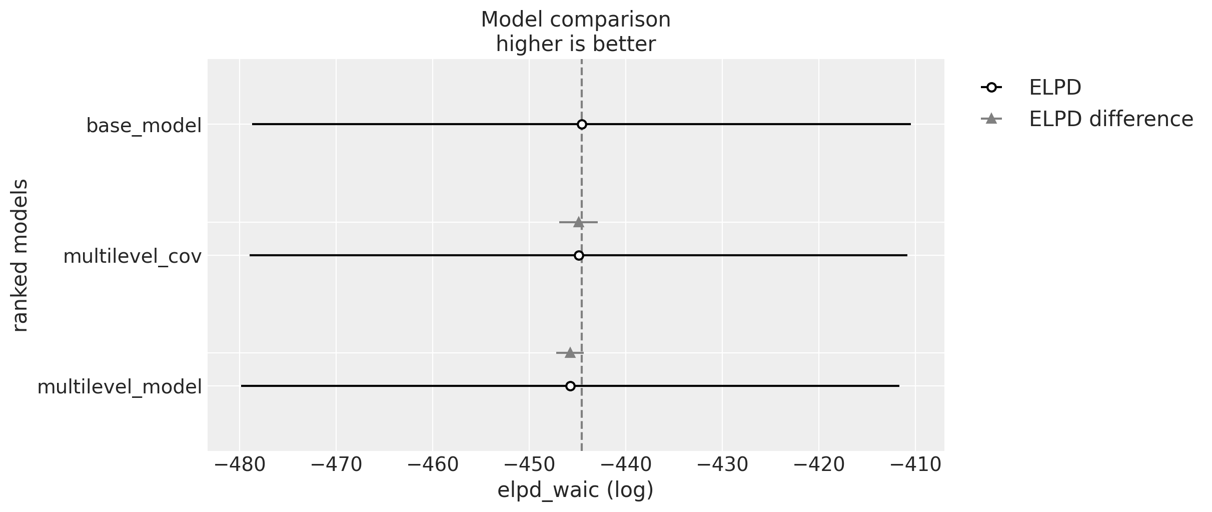
The difference between these models is minimal. It is interesting to see that the base model actually scores higher. However, as we will see below the best model for elasticity estimation is the covariance model as it allows global information to flow across regions ans samples quite fast. First let’s look into the intercepts:
ax, *_ = az.plot_forest(
    data=[idata_base, idata, idata_cov],
    model_names=["baseline", "multilevel", "cov_multilevel"],
    var_names=["alpha_j"],
    combined=True,
    figsize=(12, 7),
)
ax.set_title(
    label="Posterior Distribution of the Intercepts",
    fontsize=18,
    fontweight="bold",
)

We clearly see how the estimations move to a global mean as compared to the base model.
Finally we look into the elasticities:
ax, *_ = az.plot_forest(
    data=[idata_base, idata, idata_cov],
    model_names=["baseline", "multilevel", "cov_multilevel"],
    var_names=["beta_j"],
    combined=True,
    figsize=(12, 7),
)
ax.set_title(
    label="Posterior Distribution of the Elasticities",
    fontsize=18,
    fontweight="bold",
)
Here we can clearly see the benefits of the hierarchical and covariance model pay off: - Less noisy due the low number of stores - The estimate has lower variance.
Remark [Simulating new groups in hierarchical models]: Note that one of the benefits of hierarchical models is the ability to generate estimations for new regions as nicely described in the blog post Out of model predictions with PyMC by PyMC Labs.
Update: This was done in a second part of this notebook, see Multilevel Elasticities for a Single SKU - Part II